CS 180 Project 1: Images of the Russian Empire
Introduction
This project is inspired by the pioneering work of Sergei Mikhailovich Prokudin-Gorskii (1863–1944), who, beginning in 1907, traveled across the Russian Empire photographing people, landscapes, architecture, and industry using a three-filter (red, green, blue) technique to capture color images on glass plates. Although his vision of educational use through special projectors never came to fruition, his thousands of negatives survived and were later acquired by the Library of Congress in 1948. Today, these digitized images provide a vivid record of the final years of Imperial Russia.
Methodology
The general approach to this problem is to use the base channel—in our case, the blue channel—and then place the remaining channels, red and green, on top of it to produce the colorized version of the image. This can be done easily using slice indexing in the numpy library after converting the images to floating-point numbers. As seen from most photos downloaded from the Prokudin-Gorskii collection, a single TIFF file contains these channels in BGR order, which makes it straightforward to use functions such as numpy.dstack in Python to separate each channel and apply modifications to them.
One might decide to divide the height by 3 (assuming each channel image is the same size) and then stack the green and red channels on top of the blue channel, resulting in the following:
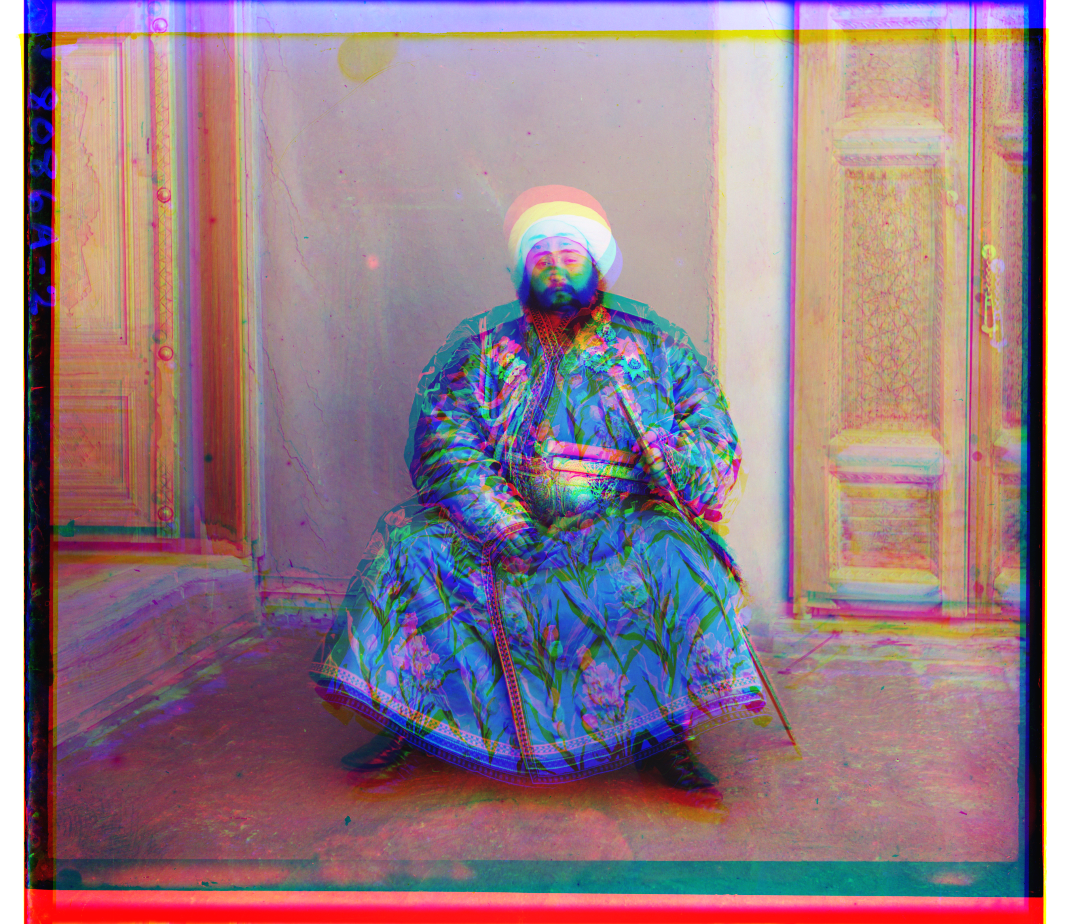
This looks quite misaligned and even dizzying if you stare at it long enough. Because the thickness of the borders of each channel image can differ, simply layering the channel images on top of each other will not work. The question then becomes: how can we align the images efficiently and effectively?
Metrics
For this project, I have only considered the simplest methods, as they already do the job perfectly for me.
\(L_1\) Norm
\[ \lVert I_1 - I_2 \rVert_{1} = \sum_{x}\sum_{y} \bigl| I_1(x,y) - I_2(x,y) \bigr| \]
Using the L1 norm to compare two images means summing the absolute differences of pixel values. It is less sensitive to large outliers than the \(L_2\) norm and tends to produce more robust alignment when a few pixels have extreme differences. This should be review from CS 189.
\(L_2\) Norm
\[ \lVert I_1 - I_2 \rVert_{2} = \sqrt{ \sum_{x}\sum_{y} \bigl( I_1(x,y) - I_2(x,y) \bigr)^2 } \]
Using the L2 norm to compare two images means summing the squares of the pixel differences and then taking the square root. It is sensitive to outliers and emphasizes larger errors more than the L1 norm, making it useful when precise alignment is desired (which can become a headache for the emir.tif image later). This should also be review from CS 189.
NCC Norm
\[ \text{NCC}(I_1, I_2) = \frac{I_1}{\lVert I_1 \rVert_2} \cdot \frac{I_2}{\lVert I_2 \rVert_2} \] where \(I_1\) and \(I_2\) are the images, and \(x\) and \(y\) are the pixel coordinates.
NCC is robust to changes in lighting and contrast, which makes it especially useful in image processing compared to standard methods like (L_1) or (L_2) norms.
Note that for the \(L_1\) and \(L_2\) norms, I inverted the values so that, for all metrics, a larger score indicates that the images are more closely aligned with each other.
All of the above metrics evaluate how similar two channel images are based on the brightness of the pixel values. For example, a pixel that is perfectly aligned should appear white, meaning that the red, green, and blue channels all have high values, regardless of their specific intensities. This approach is somewhat imperfect, as it can lead to cases where the alignment is so poor that a human can detect it without zooming in, as we will see in a few examples. But in the end, it managed to surprisingly align the pictures very well with my combination of techniques to address the issue.
Single-Scale Version
I have implemented a single-scale version of the algorithm, where the code searches over a user-specified window of displacements, with a default of (-15, 15) along both the x-axis and y-axis. The code iterates through all possible combinations of x-shifts and y-shifts, calculates the “score” based on the chosen metric, and determines which combination yields the highest score. This combination is then returned as the final best displacement according to the window defined by the user.
NCC Norm
Here are the results and the best shifts obtained using this naive approach on the images with the NCC norm:
The following command was run to generate the images:
python3 proj1.py --all_jpgs --metric = 'ncc'with default arguments alg = 'simple', search_range = 15 applied.
Processing Time: 1.34 s
Best Shift: G = [1, 7], R = [3, 12]

Processing Time: 1.45 s
Best Shift: G = [1, 6], R = [2, 3]

Processing Time: 1.38 s
Best Shift: G = [1, 4], R = [3, 6]
\(L_2\) Norm
Here are the results and the best shifts obtained using this naive approach on the images with the \(L_2\) norm:
The following command was run to generate the images:
python3 proj1.py --all_jpgswith default arguments alg = 'simple', search_range = 15, metric = l2 applied.
Processing Time: 0.34 s
Best Shift: G = [1, 7], R = [3, 12]

Processing Time: 0.38 s
Best Shift: G = [1, 6], R = [2, 3]

Processing Time: 0.32 s
Best Shift: G = [1, 4], R = [3, 6]

(It’s not a coincidence, nor me being lazy, that the data shown above for the images looks the same across metrics — the algorithm is simple enough, the images are simple enough, and the metrics are good enough that the shifts end up nearly identical. In fact, the only real difference is the processing time, which makes sense since NCC, relatively speaking, involves more arithmetic operations. For example, we’ll see this remains true for the \(L_1\) norm as well.)
\(L_1\) Norm
Here are the results and the best shifts obtained using this naive approach on the images with the \(L_1\) norm:
The following command was run to generate the images:
python3 proj1.py --all_jpgs --metric l1with default arguments alg = 'simple', search_range = 15 applied.
Processing Time: 0.46 s
Best Shift: G = [1, 7], R = [3, 11]

Processing Time: 0.47 s
Best Shift: G = [1, 6], R = [2, 3]

Processing Time: 0.42 s
Best Shift: G = [1, 4], R = [3, 6]

As a side observation, it seems that NCC, \(L_2\), and \(L_1\) all perform equally well in this single-scale version of the algorithm. I think this is mainly because, first, the resolutions of the images are not high enough to make it ambiguous what might be a better alignment, and second, the size of the user-defined search window does not significantly affect the final result.
Pyramid-Speedup Version
Exhaustive search will become prohibitively expensive if there are too many pixels within an image, for exampels those tilf images. So I developed this speed up algorithim.
Cropping
In addition to the processing step where we split the image into different color channels, the first new step we will take is to crop the images. For now, this is done manually, with users able to set crop_percent. I found 5% to work best, so that will be the default. This step was crucial for my project because, once implemented, the images aligned much better and the algorithm performed significantly improved. The black borders of the images were negatively affecting the results for some reason.
Downscaling
In addition to splitting the image into different color channels, the first new step is to downscale the images so that we can efficiently run, for example, our single-scale version on them. This method works well on smaller images, though it can be computationally expensive for larger ones.
Inspired by the average pooling layers in CNNs taught in CS189, we downscale by taking the average of every factor \(\times\) factor pixels (where factor is user-settable, with a default value of 2). Unlike naive pooling in CNNs, each pixel is counted only once (in CNNs, a pixel can contribute to multiple overlapping regions). If the image dimensions are not evenly divisible by factor, we trim the image accordingly.
We then recursively downscale the image until its height is at most starting_scale, which can also be set by the user (default: 100).
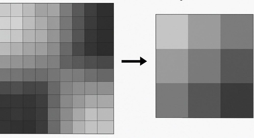
We can also implement a simpler version where we either keep only the top-left pixel of each square or take the maximum or minimum value. However, I prefer the averaging approach, so I will stick with that.
Localized Optimization
Performing a full search over a large user-defined window (defaulting from -15 to 15) can take a long time on large images—sometimes more than a minute! To make this more efficient, we instead set a small search_range, typically between 2 and 5.
Starting from the coarsest downscaled version of the image, we perform a localized search using our single-scale version of the algorithm (defaulting to a -5 to 5 grid window) to find the best shift parameters. Next, we upscale the image by 2× and scale the current shift parameters by 2. We then refine the shift parameters after applying the current shift to the upscaled image. In other words, the image is progressively shifted, and the shift size is gradually increased as we move to finer resolutions.
We repeat this process until we reach the original image size. The result is a set of locally optimized shifting parameters. As learned in CS189, this approach is similar to forward feature selection: choosing the best step at each stage does not guarantee a globally optimal solution, but in our case, it is sufficient to achieve excellent alignment quickly.
Gallery and Results
NCC Metric
The following command was run to generate the images:
python3 proj1.py --all_tifswith default arguments alg = 'complex', search_range = 3, metric = 'ncc', crop_percent = 0.05, starting_scale = 100 applied.
| Image | Green Channel Displacement | Red Channel Displacement | Processing Time (s) |
|---|---|---|---|
 |
(17, 57) | (44, 103) | 11.81 |
 |
(15, 39) | (35, 77) | 12.82 |
 |
(-7, 33) | (-4, 58) | 13.62 |
 |
(-2, 58) | (9, 112) | 11.91 |
 |
(-12, 52) | (-28, 92) | 12.42 |
 |
(3, 96) | (12, 178) | 12.37 |
 |
(-7, 78) | (-8, 76) | 12.26 |
| (5, 48) | (23, 89) | 12.40 | |
 |
(-18, 46) | (-25, 95) | 12.68 |
 |
(8, 98) | (36, 176) | 12.91 |
 |
(-3, 65) | (13, 124) | 12.24 |
 |
(1, 7), (3, 12), 0.18s | (1, 7), (3, 12), 0.09s | (1, 7), (3, 9), 0.09s |
 |
(1, 4), (3, 6), 0.19s | (1, 4), (3, 6), 0.08s | (1, 4), (3, 6), 0.06s |
 |
(1, 6), (2, 3), 0.14s | (1, 6), (2, 3), 0.07s | (1, 6), (2, 3), 0.09s |
Below are the bonus images to which I applied the algorithm:
| Image | Green Channel Displacement | Red Channel Displacement | Processing Time (s) |
|---|---|---|---|
 |
(-14, 74) | (-17, 126) | 12.00 |
 |
(-7, 69) | (-2, 133) | 12.07 |
 |
(-31, 42) | (-40, 82) | 12.03 |
\(L_2\) Metric
The following command was run to generate the images:
python3 proj1.py --all_tifs --metric 'l2' --crop_percent 0.1with default arguments alg = 'complex', search_range = 3, starting_scale = 100 applied.
| Image | Green Channel Displacement | Red Channel Displacement | Processing Time (s) |
|---|---|---|---|
 |
(17, 57) | (42, 100) | 2.77 |
 |
(15, 38) | (35, 76) | 2.76 |
 |
(-8, 33) | (-4, 58) | 3.91 |
 |
(-3, 58) | (11, 111) | 3.08 |
 |
(-13, 52) | (-29, 92) | 3.51 |
 |
(3, 96) | (13, 178) | 3.05 |
 |
(-7, 78) | (-3, -3) | 3.28 |
| (5, 48) | (23, 89) | 3.10 | |
 |
(-18, 47) | (-25, 96) | 4.15 |
 |
(8, 98) | (37, 176) | 3.91 |
 |
(-3, 65) | (13, 123) | 3.18 |
 |
(1, 7) | (3, 12) | 0.09 |
 |
(1, 4) | (3, 6) | 0.08 |
 |
(1, 6) | (2, 3) | 0.07 |
Bonus:
| Image | Green Channel Displacement | Red Channel Displacement | Processing Time (s) |
|---|---|---|---|
 |
(-13, 74) | (-13, 125) | 3.12 |
 |
(-8, 69) | (-2, 133) | 3.86 |
 |
(-31, 41) | (-39, 82) | 3.38 |
(Note again: the \(L_2\) norm doesn’t actually change the results from the NCC norm that much in this case, but you can see that the processing times differ. With my algorithm, unless someone proposes a significantly better or worse method, it’s hard for the displacement values to change much.)
\(L_1\) Metric
The following command was run to generate the images:
python3 proj1.py --all_tifs --metric 'l1'with default arguments alg = 'complex', search_range = 3, crop_percent = 0.05, starting_scale = 100 applied.
| Image | Green Channel Displacement | Red Channel Displacement | Processing Time (s) |
|---|---|---|---|
 |
(17, 57) | (42, 104) | 4.68 |
 |
(14, 39) | (35, 76) | 4.64 |
 |
(-8, 33) | (-4, 58) | 4.33 |
 |
(-3, 59) | (9, 112) | 4.52 |
 |
(-12, 51) | (-29, 92) | 4.67 |
 |
(3, 96) | (13, 178) | 4.66 |
 |
(-7, 78) | (-7, 77) | 4.58 |
| (5, 48) | (22, 90) | 4.78 | |
 |
(-18, 47) | (-26, 97) | 4.97 |
 |
(8, 98) | (36, 175) | 4.83 |
 |
(-3, 65) | (14, 124) | 4.62 |
 |
(1, 7) | (3, 9) | 0.09 |
 |
(1, 4) | (3, 6) | 0.06 |
 |
(1, 6) | (2, 3) | 0.09 |
Bonus:
| Image | Green Channel Displacement | Red Channel Displacement | Processing Time (s) |
|---|---|---|---|
 |
(-13, 74) | (-19, 126) | 4.73 |
 |
(-7, 70) | (-1, 133) | 4.58 |
 |
(-28, 43) | (-38, 83) | 4.60 |
Summary
| Image | NCC (G, R, Time) | \(L_2\) (G, R, Time) | \(L_1\) (G, R, Time) |
|---|---|---|---|
|
(17, 57), (44, 103), 11.81s | (17, 57), (42, 100), 2.77s | (17, 57), (42, 104), 4.68s |
|
(15, 39), (35, 77), 12.82s | (15, 38), (35, 76), 2.76s | (14, 39), (35, 76), 4.64s |
|
(-7, 33), (-4, 58), 13.62s | (-8, 33), (-4, 58), 3.91s | (-8, 33), (-4, 58), 4.33s |
|
(-2, 58), (9, 112), 11.91s | (-3, 58), (11, 111), 3.08s | (-3, 59), (9, 112), 4.52s |
|
(-12, 52), (-28, 92), 12.42s | (-13, 52), (-29, 92), 3.51s | (-12, 51), (-29, 92), 4.67s |
|
(3, 96), (12, 178), 12.37s | (3, 96), (13, 178), 3.05s | (3, 96), (13, 178), 4.66s |
|
(-7, 78), (-8, 76), 12.26s | (-7, 78), (-3, -3), 3.28s | (-7, 78), (-7, 77), 4.58s |
| (5, 48), (23, 89), 12.40s | (5, 48), (23, 89), 3.10s | (5, 48), (22, 90), 4.78s | |
|
(-18, 46), (-25, 95), 12.68s | (-18, 47), (-25, 96), 4.15s | (-18, 47), (-26, 97), 4.97s |
|
(8, 98), (36, 176), 12.91s | (8, 98), (37, 176), 3.91s | (8, 98), (36, 175), 4.83s |
|
(-3, 65), (13, 124), 12.24s | (-3, 65), (13, 123), 3.18s | (-3, 65), (14, 124), 4.62s |
|
(-14, 74), (-17, 126), 12.00s | (-13, 74), (-13, 125), 3.12s | (-13, 74), (-19, 126), 4.73s |
|
(-7, 69), (-2, 133), 12.07s | (-8, 69), (-2, 133), 3.86s | (-7, 70), (-1, 133), 4.58s |
|
(-31, 42), (-40, 82), 12.03s | (-31, 41), (-39, 82), 3.38s | (-28, 43), (-38, 83), 4.60s |
|
(1, 7), (3, 12), 0.18s | (1, 7), (3, 12), 0.09s | (1, 7), (3, 9), 0.09s |
|
(1, 4), (3, 6), 0.19s | (1, 4), (3, 6), 0.08s | (1, 4), (3, 6), 0.06s |
|
(1, 6), (2, 3), 0.14s | (1, 6), (2, 3), 0.07s | (1, 6), (2, 3), 0.09s |
Overall, my algorithm performs extremely well on the images while maintaining very fast processing speeds (note that the processing time even includes generating images from floats, which means the algorithm itself took even less time to run). It is also fairly straightforward.
Problems Encountered
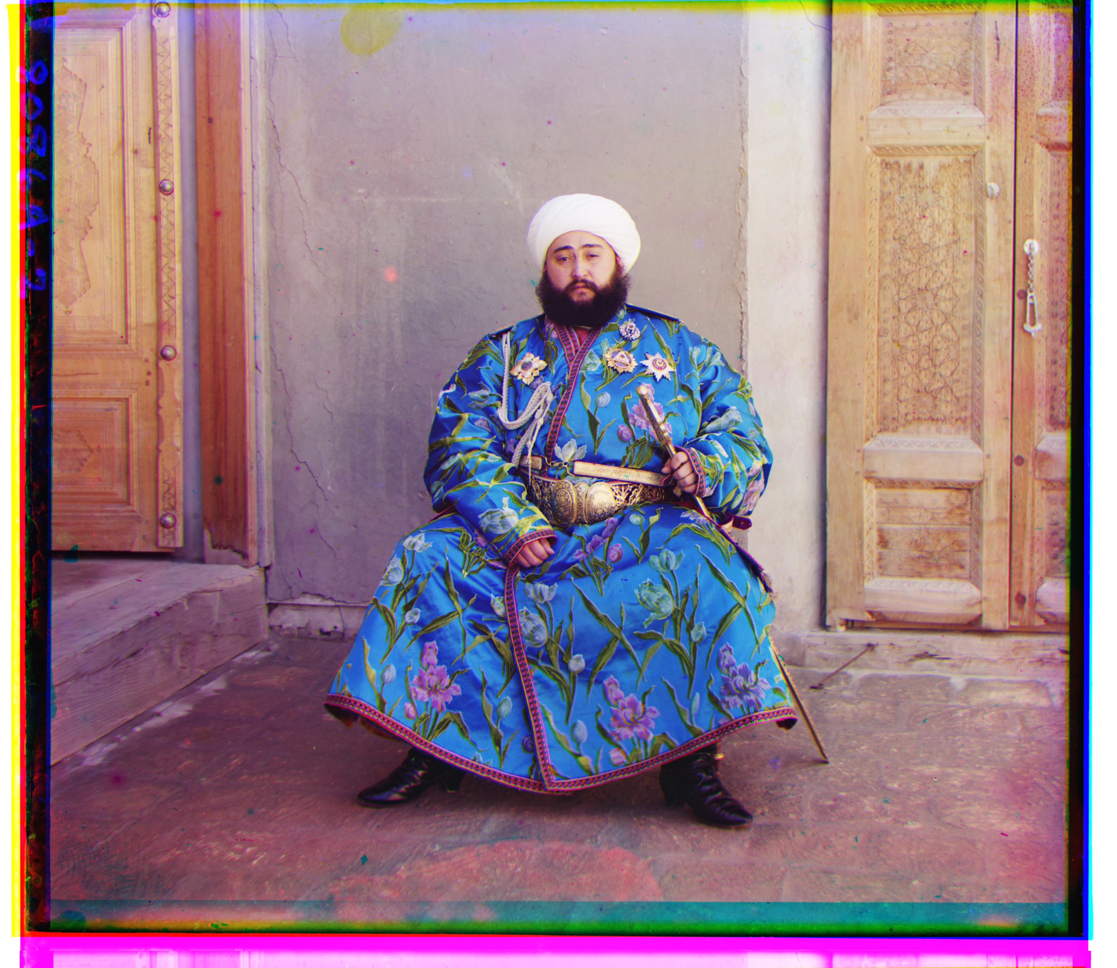
Interestingly enough, I managed to have the emir.tif file converted to a JPG image, which showed that he was wearing an orange dress when I first did the assignment! That couldn’t really be the case, I told myself—only later did I realize that I had been assigning the image to the wrong color channels, which caused such strange coloring.
Another issue, as hinted above, was that I didn’t consider cutting the borders, which literally destroyed the algorithm’s performance. I couldn’t get the images to look the way I wanted, but after that simple tweak, everything worked perfectly.
The emir.tif image was the toughest to work with. As the hint suggested, one would likely need edge detectors in their code to make things easier. However, I found that cropping the borders significantly improved my image alignment, so I managed without using them.