CS 180 Project 4: Neural Radiance Field
In this project, we will explore how we can use a NeRF model to generate cool novel views from 360 degrees.
Part 0: Calibrating Your Camera and Capturing a 3D Scan
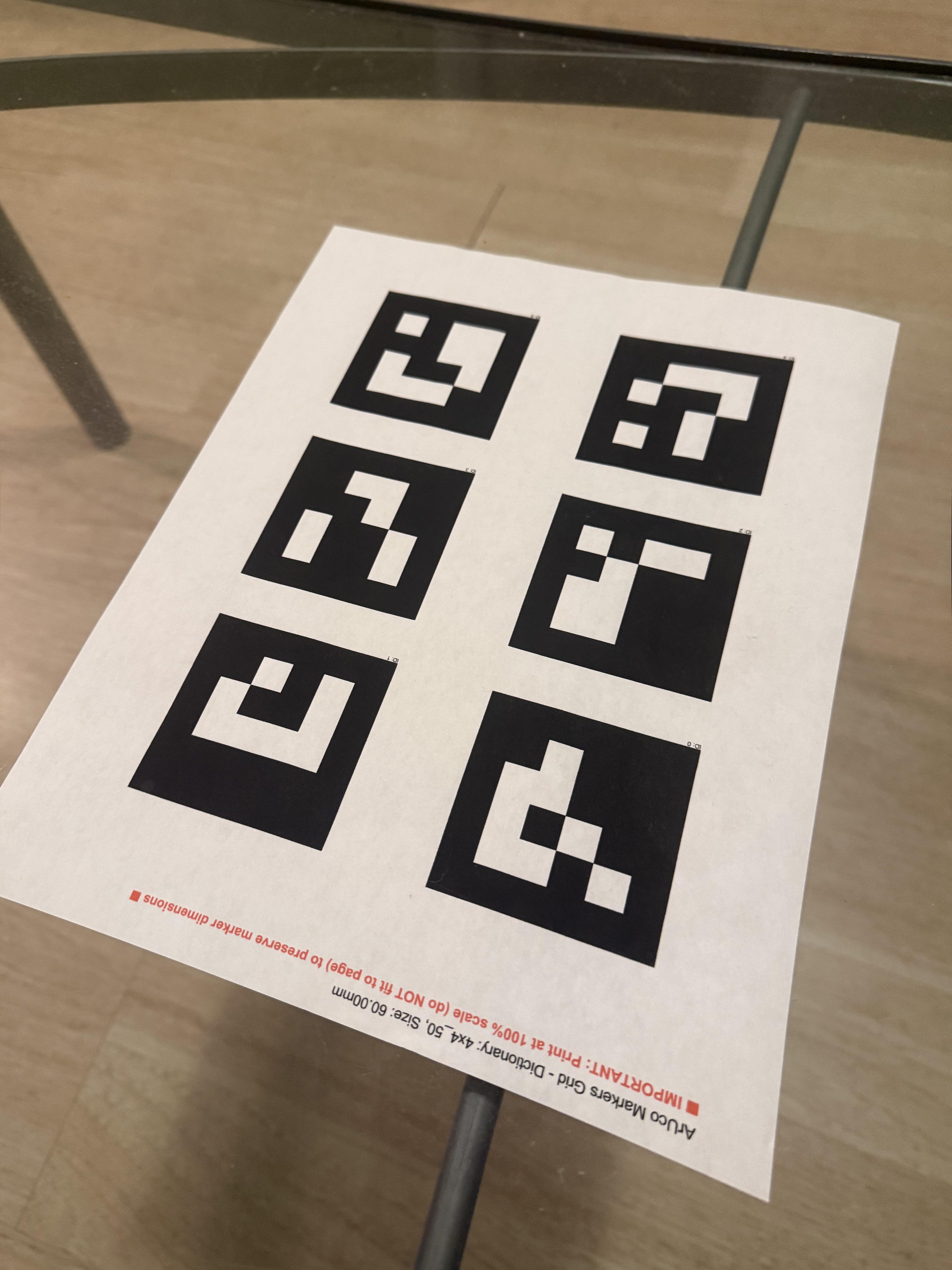
For the first part, I will take a 3D scan of my own object using visual tracking targets called ArUco tags.
Part 0.1: Calibrating Your Camera
ArUco tags are useful, as the opencv Python package provides some cool functions that can help us learn the specifics of our cameras without actually having to calculate them from elsewhere.
Initially, we planned to take roughly 50 images for this purpose, so we could capture the information about our camera, and aim to have a reconstruction error less than 1. As I kept debugging in this project, I was instead taking 170 images of the tags, and disregarding some of the troublemaking or outlier ones. I eventually ended up with 35 filtered images that I believe to be the best based on the mean error comparing the reconstructed images (and as I am writing this sentence, the reconstruction error is around 3.5).
The following are some images I took for this purpose:
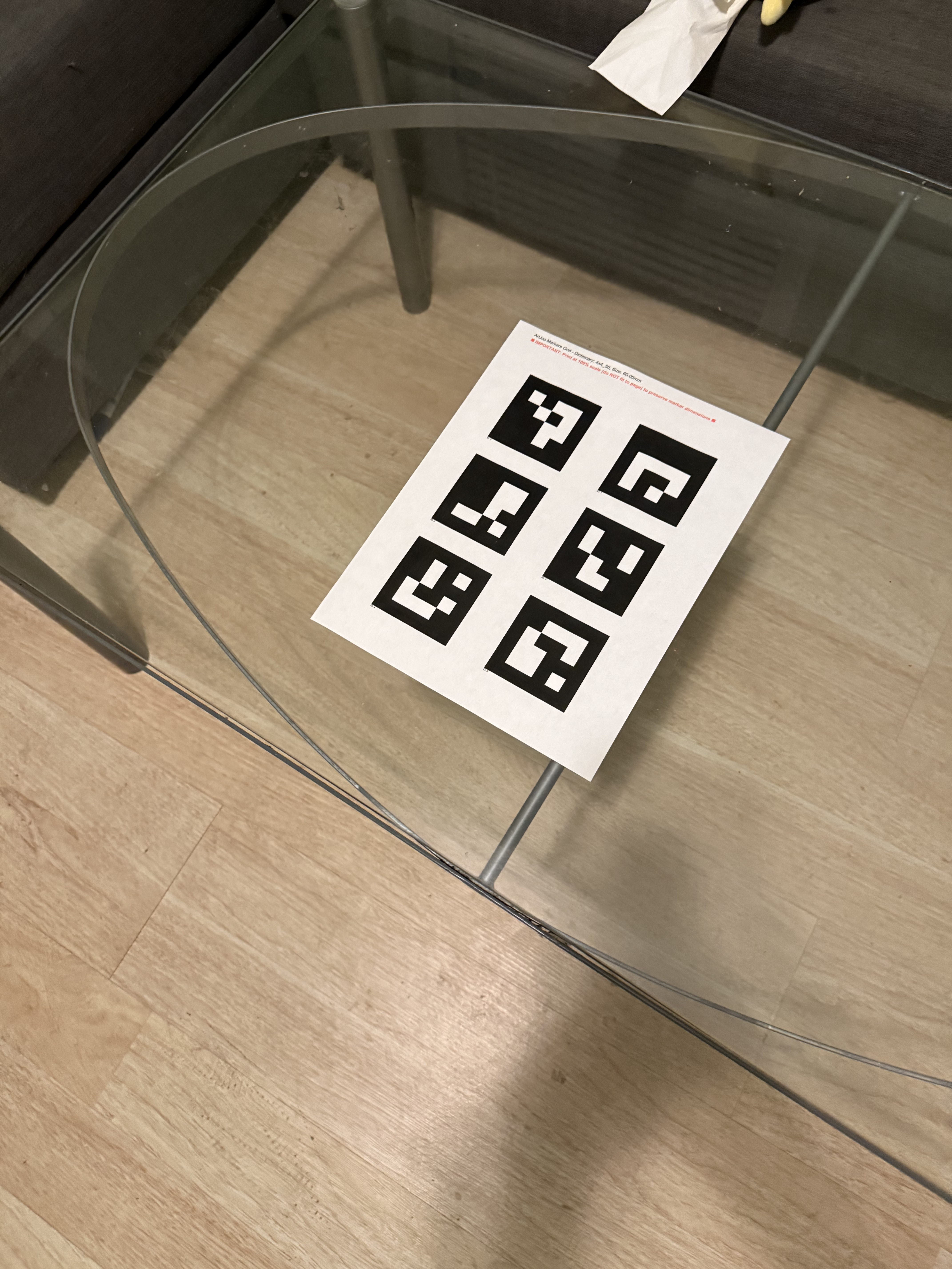
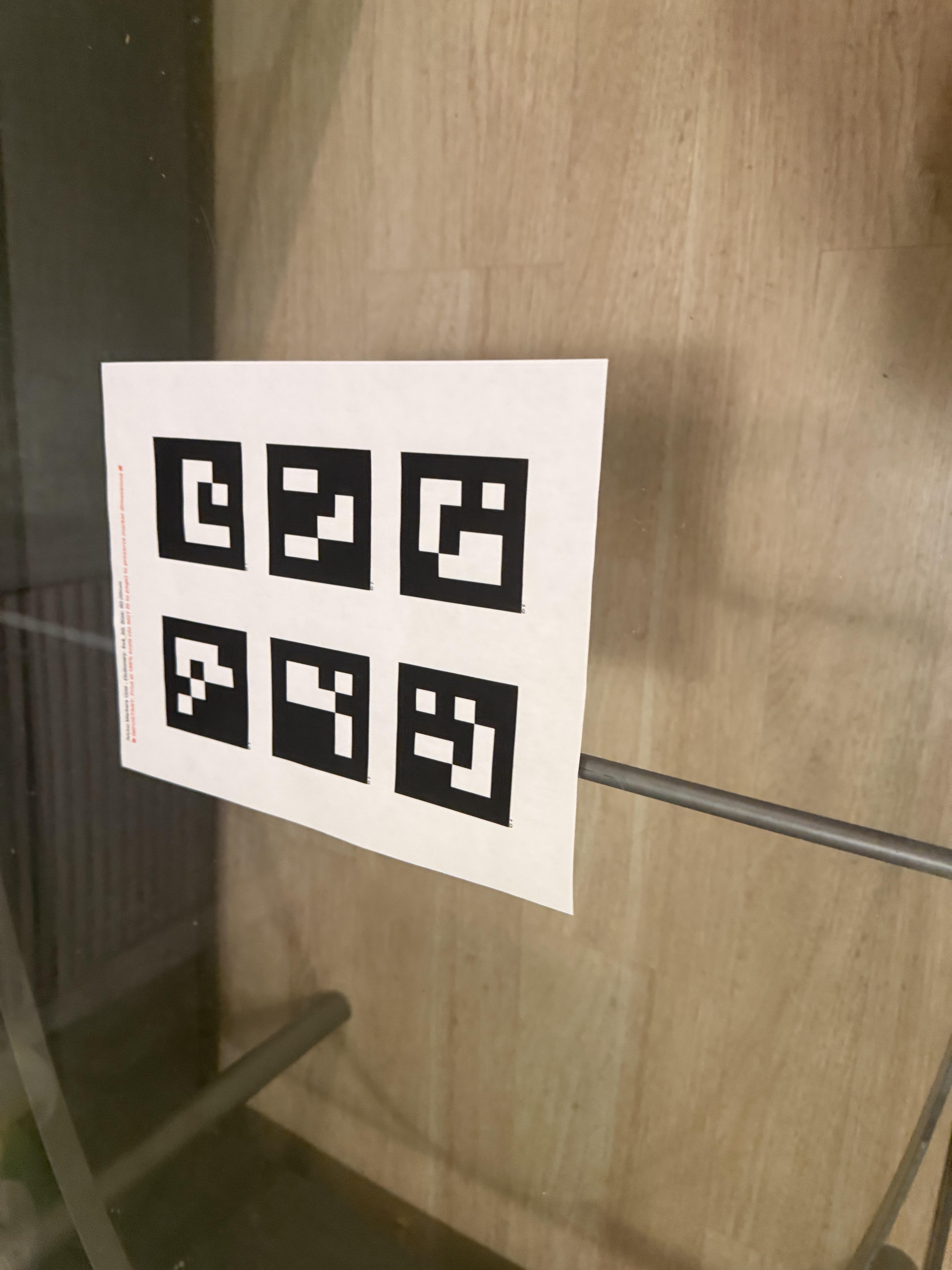
As seen, tags are taken from different angles and different distances to make sure we roughly have the best camera parameters without taking more pictures.
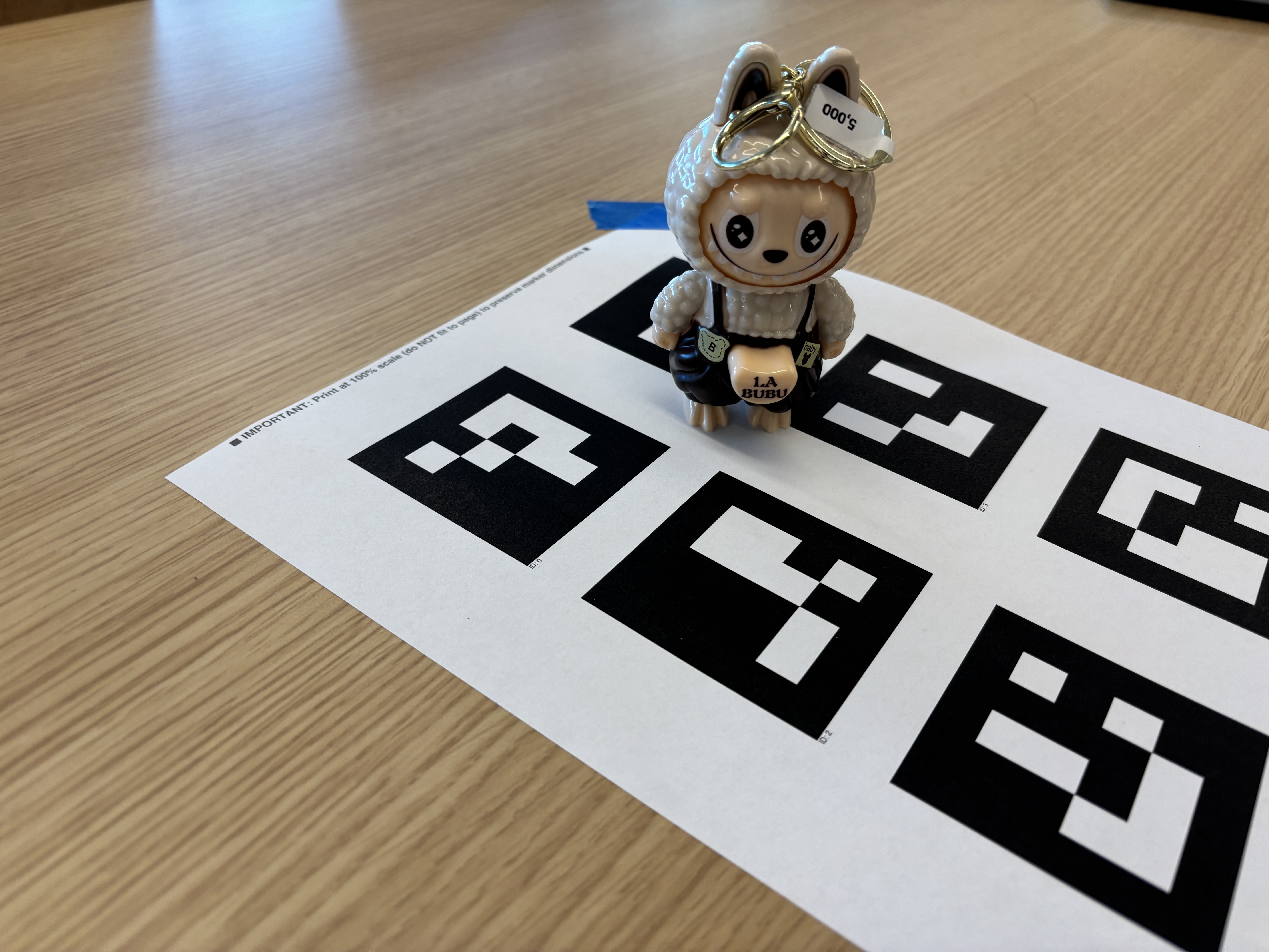
Part 0.2: Capturing a 3D Object Scan
Now we will be taking some pictures of our object that we want to record a novel 360 degree view of it. For this project I tried two different items, one which is a plushie that is probably 30cm long and also an airtag case that is around 5cm long. I ultimately chose to go with the latter one, as it seems most related to the lafufu presented in the example given by course staff.
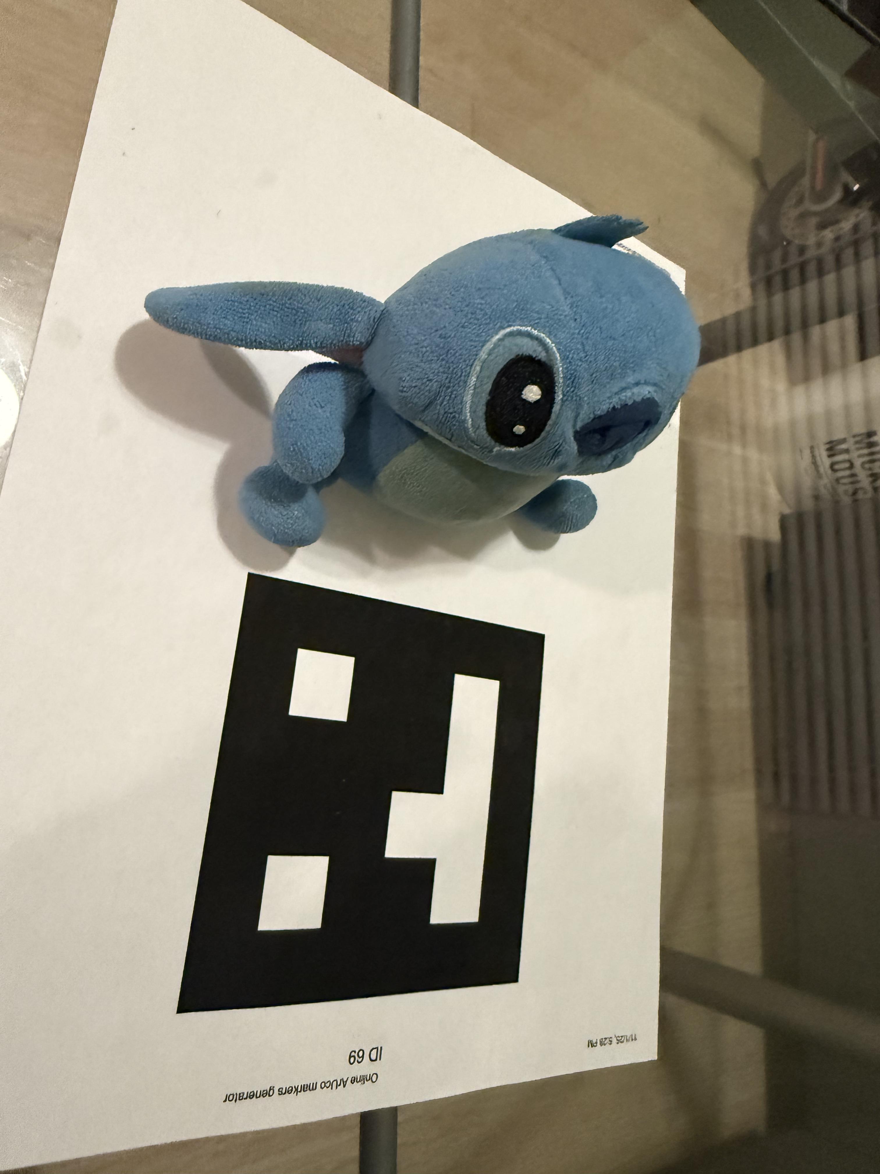
Note that in contrast, I am using a single ArUco tag, while the course staff is using 6 of them on a single piece of paper. This is intentional, as we were instructed that way.
Part 0.3: Estimating Camera Pose
To make sure we aren’t messing anything up, we will be estimating the camera poses on these lovely objects to make sure that their relative positions make sense in the 3D space.
The following two images are some images I captured in this process:
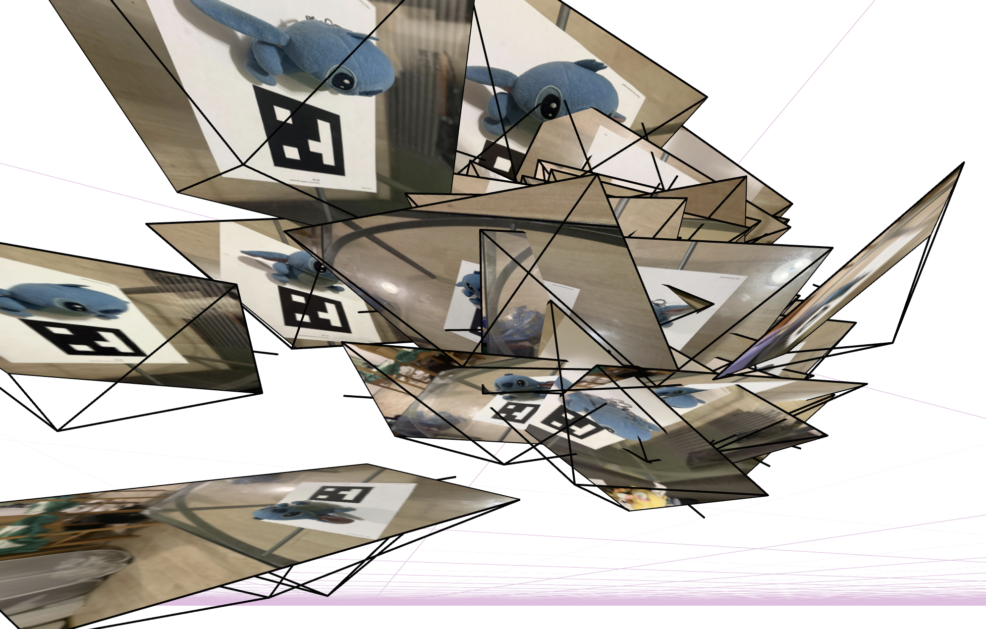
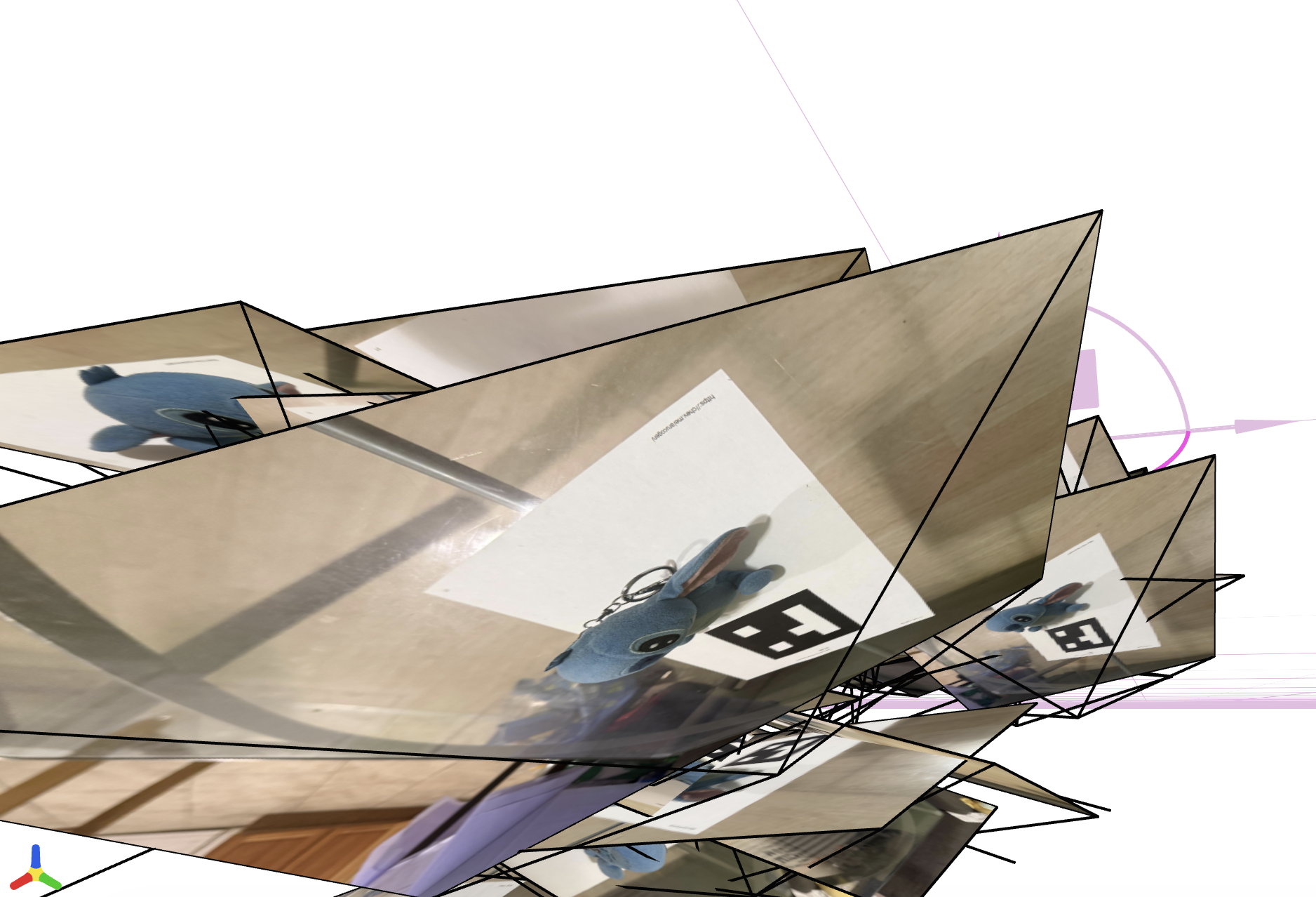
Though it looks a bit different from the ideal one, I believe this is because of how I swapped the z-axis, which makes it very hard to visualize what is actually going on among the different cameras. According to some discussions I posted and later images that we will see in a bit, this seems fine.
Part 0.4: Undistorting images and creating a dataset
To prepare our dataset for later steps, we will undistort our images to make sure straight lines look straight, so we don’t have to worry about the dataset being the root cause for messing up the NeRF model.
Below is an example of the undistorted image:
Note that I am pretty confident with the quality of the image. Hence, you won’t see that much difference between the original image and this undistorted image (images that seem to be messed up most likely have been eliminated when we filtered them out earlier).
Part 1: Fit a Neural Field to a 2D Image
Before jumping into our NeRF model for 3D objects, we will start simple with a 2D image. We will train a neural network to fit two images: one is the reference dog image provided, and one is a fox image of my own.
Model Architecture
Our model consists of:
- MLP: 4 layers (depth = 4) with width of either 16, 64, or 128, depending on whether we are testing for hyperparameter exploration
- Positional Encoding: Max frequency parameter \(L\) of 2, 5, or 10 depending on whether we are doing hyperparameter exploration
- Input dimension: \(2 + 4 \times L\) (e.g., \(L=10\) gives in_dim = 42)
- Learning Rate: 0.01
- Batch Size: 10,000 random pixels per iteration
- Training Iterations: 2,000
- Activation: ReLU for hidden layers, Sigmoid for output layer (to clamp RGB values to [0,1])
The network takes 2D coordinates \((x, y)\) normalized to \([0, 1]\) as input, applies positional encoding, and outputs RGB values for each pixel.
Training Progression
Dog Image
The following shows the training progression on the provided dog.png image (his name is Taroumaru!) at different iterations:

Fox Image
The following shows the training progression on the provided fox.jpg image at different iterations:
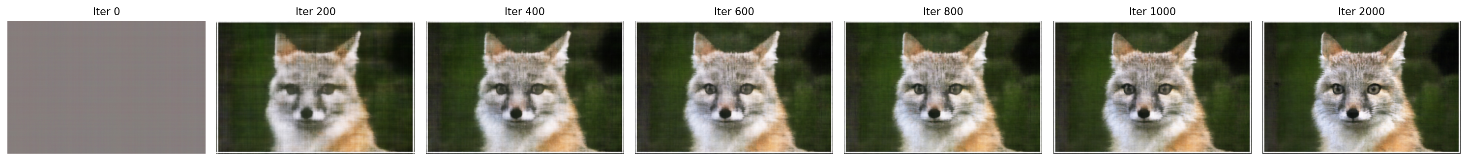
As can be seen from both progressions, the network starts from a random initialization and gradually learns to reconstruct the image, with significant improvement in the first few hundred iterations and continued refinement throughout training.
Hopefully this will be the pattern we will see when we move to 3D objects.
2×2 Grid: Hyperparameter Comparison
To analyze the effect of different hyperparameters, we trained the model with 2 choices of positional encoding frequency (L=2, L=5) and 2 choices of network width (16, 64), creating a 2×2 grid of results using low values to better observe their impact:
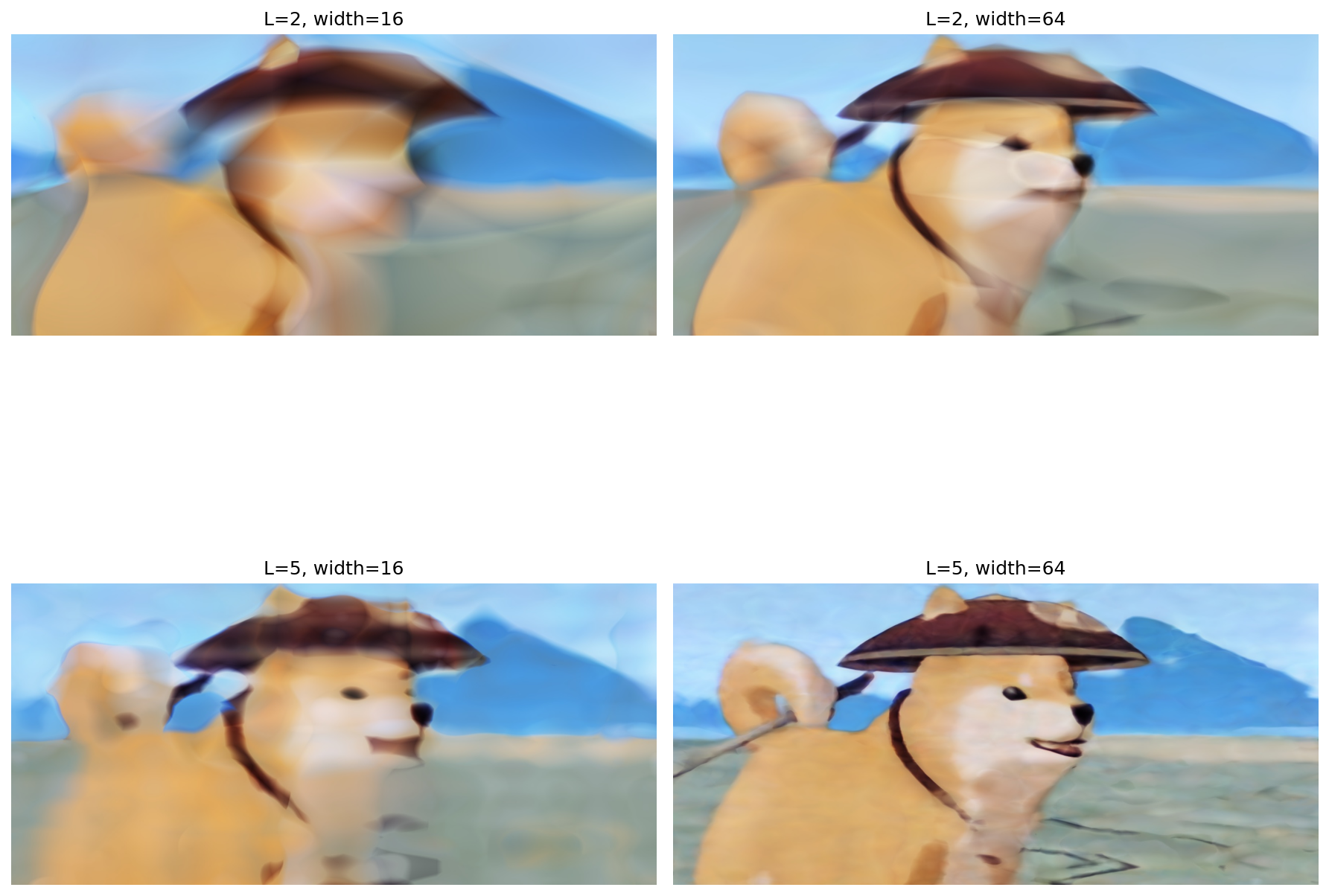
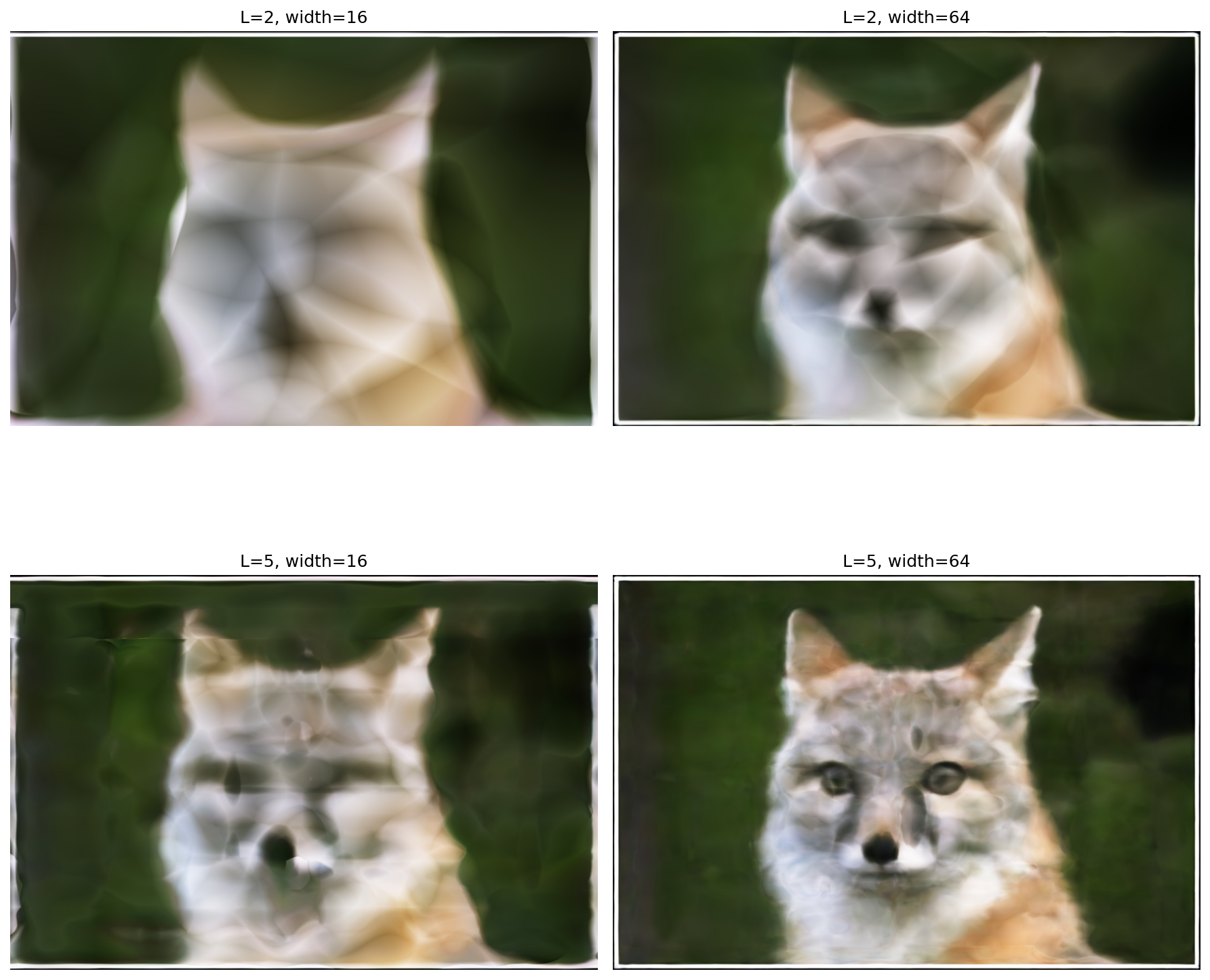
As we can see above, it seems like as long as we increase \(L\) and \(W\), we can get a very good estimation or reconstruction of the original image, which makes sense. In neural networks, if you have more parameters, you can learn more about the pattern and get a better result.
In more detail:
- Lower \(L\): Results in less detailed reconstructions as the positional encoding has fewer frequency components, which limits the network’s ability to capture high-frequency details.
- Higher \(L\): Allows for better detail capture, though still limited compared to default \(L=10\).
- Lower width: Smaller network capacity leads to smoother but less detailed outputs.
- Higher width: More network capacity enables better reconstruction quality, though with some artifacts.
The hyperparameters significantly affect the network’s ability to capture fine details and sharp edges in the image.
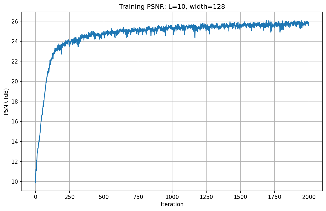
PSNR Curve
The following shows the PSNR curve during training on the fox image with default hyperparameters:
Similarly, we can also see how it performs on our own dog image with default hyperparameters:
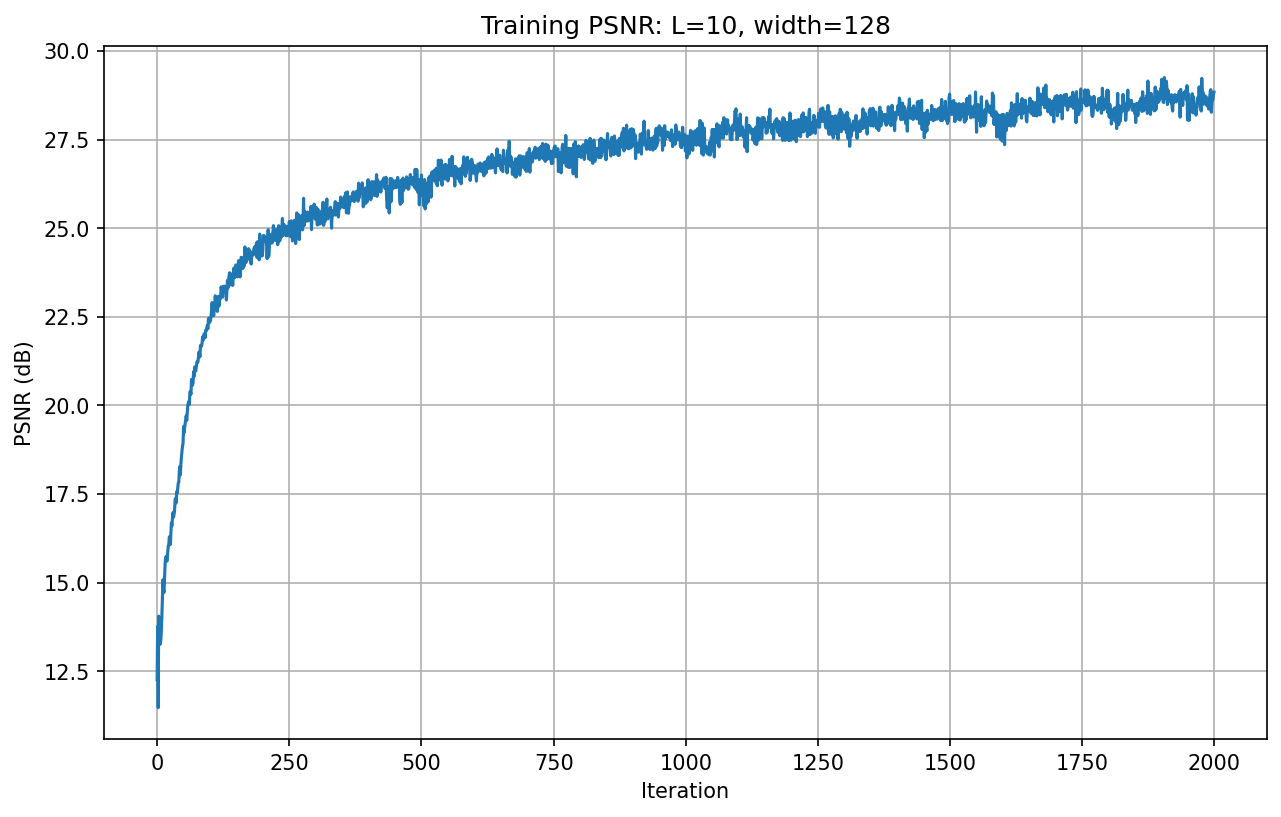
The PSNR increases rapidly in the first few hundred iterations, then continues to improve gradually, reaching a final PSNR of approximately 28.7 dB after 2000 iterations.
Comparatively speaking, the dog image that I found and decided to reconstruct had a better chance to be reconstructed and achieve better PSNR, possibly because the lighting and pixel values are easier to recognize and recreate.
Part 2: Fit a Neural Radiance Field from Multi-view Images
In this part, as we got familiar with the NeRF model with 2D objects, we will start the actual NeRF model with 3D objects.
Part 2.1: Create Rays from Cameras
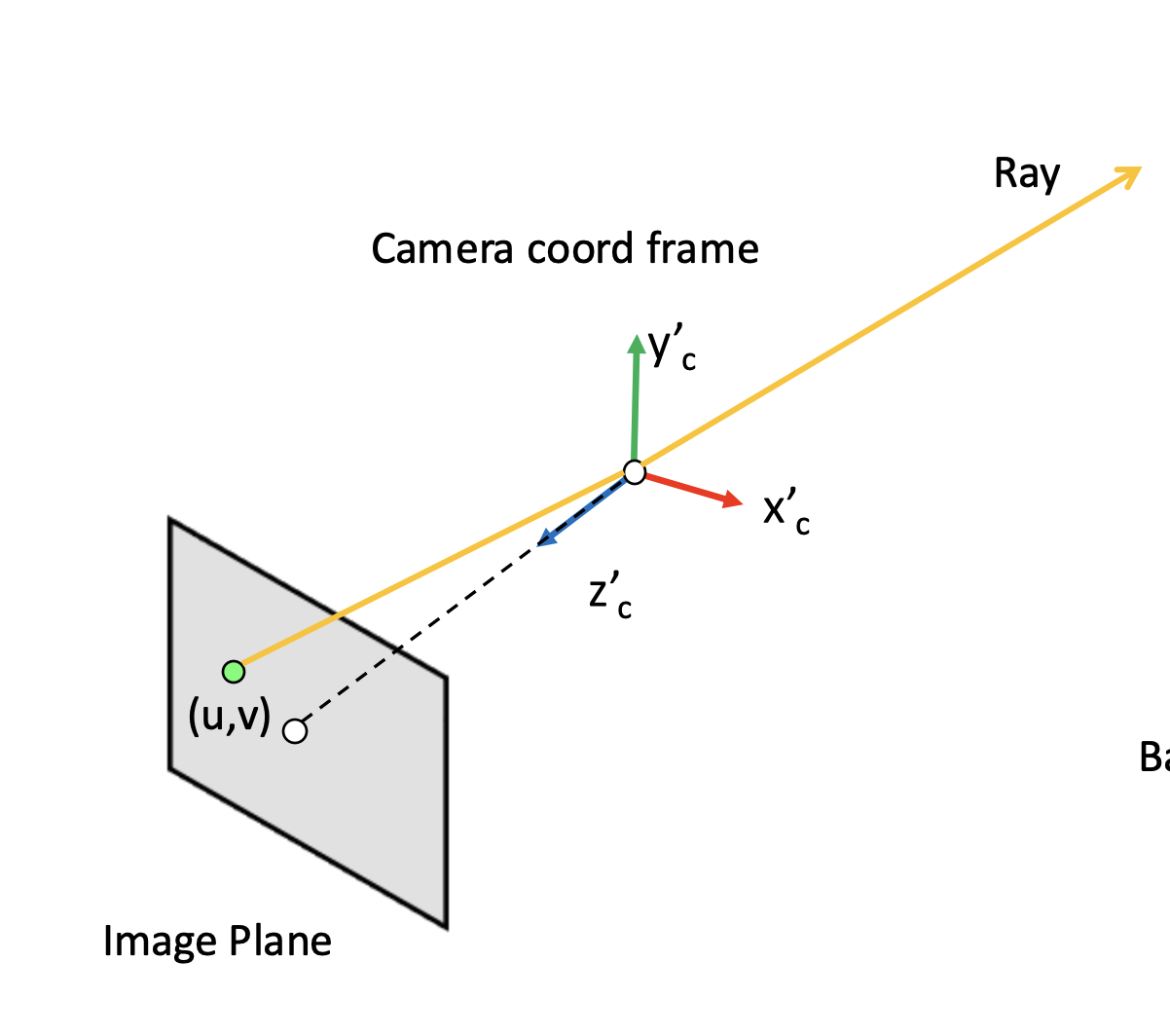
We have the camera coordinates. We want the pixel values along the rays when we are shooting from the camera, and basically want to train a neural network based on this so that no matter if we actually had a camera at that position aiming at that angle in the first place, we would like to recreate it. In the lecture, the following diagram was presented which might be useful for this:
 {width=“80%”, fig-align=“center”}
From camera to world coordinates, we will be using the very familiar equations that we have been using in the previous project:
\[\begin{align} \begin{bmatrix} x_c \\ y_c \\ z_c \\ 1 \end{bmatrix} = \begin{bmatrix} \mathbf{R}_{3\times3} & \mathbf{t} \\ \mathbf{0}_{1\times3} & 1 \end{bmatrix} \begin{bmatrix} x_w \\ y_w \\ z_w \\ 1 \end{bmatrix} \end{align}\]
We implement it by: (1) converting the point to homogeneous coordinates, (2) multiplying by the camera-to-world matrix c2w, and (3) converting back to 3D.
Additionally, we will also have a function that helps us convert from pixel to camera coordinates:
\[\begin{align} \mathbf{K} = \begin{bmatrix} f_x & 0 & o_x \\ 0 & f_y & o_y \\ 0 & 0 & 1 \end{bmatrix} \end{align}\]
Similarly, we: (1) create homogeneous pixel coordinates \((u, v, 1)\), (2) apply the inverse camera intrinsics \(\mathbf{K}^{-1}\), and (3) scale by a depth value \(s\).
What is more interesting is pixel to ray coordinates, since this is what NeRF is heavily based on:
\[\begin{align} \mathbf{r}_d = \frac{\mathbf{X_w} - \mathbf{r}_o}{||\mathbf{X_w} - \mathbf{r}_o||_2} \end{align}\]
Similarly, we will: (1) extract the camera’s world-space position as the ray origin \(\mathbf{r}_o\), (2) convert the pixel to a camera-space point via pixel_to_camera, (3) transform that point to world space via transform, and (4) compute the normalized ray direction \(\mathbf{r}_d\) from origin to that point.
Part 2.2: Sampling
To train the NeRF models, we will sample some rays among the images so that the NeRF model can actually learn the patterns in the environment that the cameras are surrounding. Along those rays, we will also sample some pixel values (since rays are technically infinitely long, or there are technically infinite points along the rays)!
To implement this, we will: (1) randomly select img_idxs and pixel coordinates \((u, v)\) within each image, (2) retrieve the corresponding camera pose c2w and the pixel color at those coordinates. To sample points along the ray, we will: (1) create 64 evenly spaced depth values per ray, (2) compute midpoints, then add random perturbation for stratified sampling, and (3) convert depths into 3D sample points.
Part 2.3: Putting the Dataloading All Together
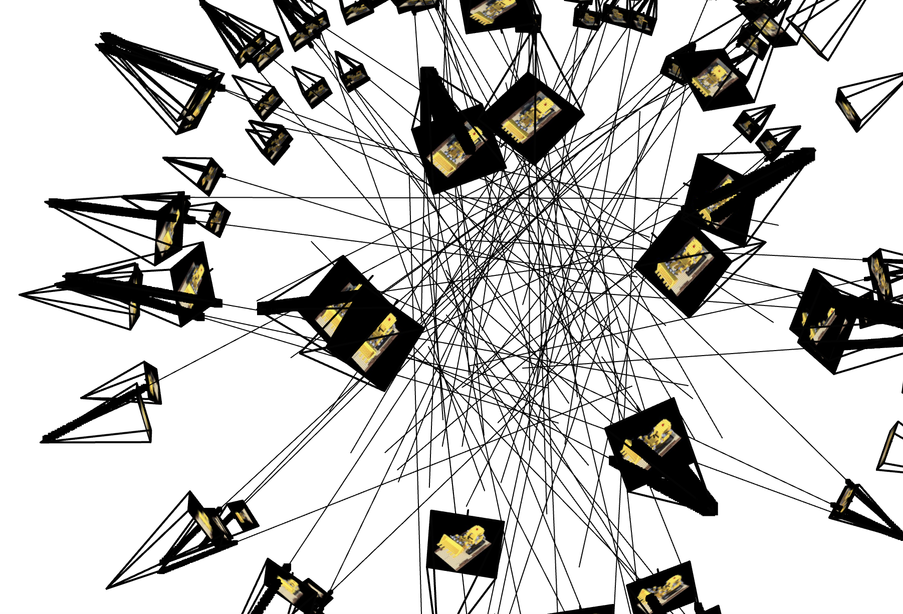
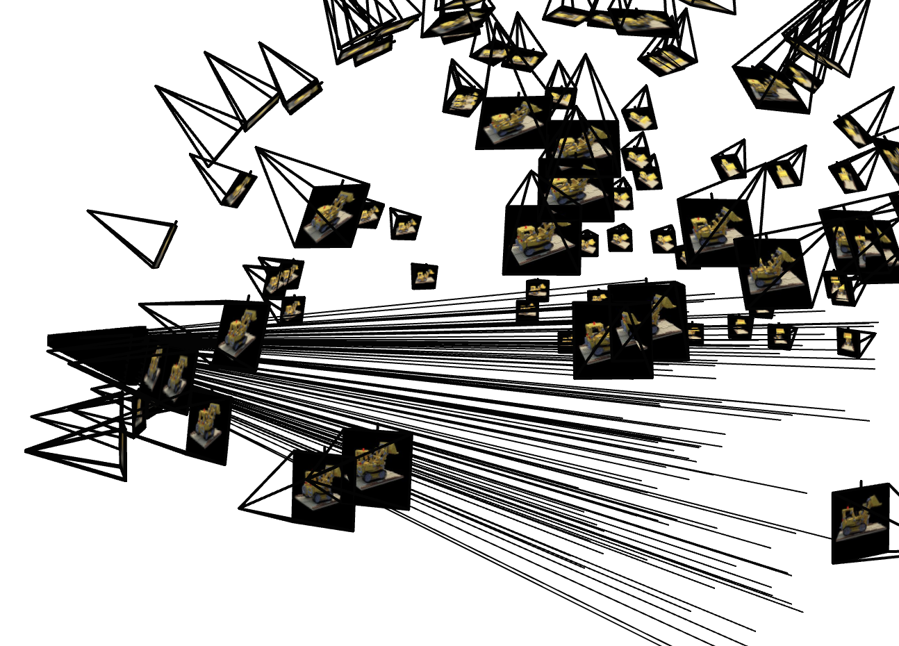
To train the model, we have also implemented the dataloader. To check whether our current implementation is correct, we have used the test code provided in the skeleton code. The results are shown below:
The test code is shown below:
# --- You Need to Implement These ------
dataset = RaysData(images_train, K, c2ws_train)
rays_o, rays_d, pixels = dataset.sample_rays(100) # Should expect (B, 3)
points = sample_along_rays(rays_o, rays_d, perturb=True)
H, W = images_train.shape[1:3]
# ---------------------------------------

server = viser.ViserServer(share=True)
for i, (image, c2w) in enumerate(zip(images_train, c2ws_train)):
    server.add_camera_frustum(
        f"/cameras/{i}",
        fov=2 * np.arctan2(H / 2, K[0, 0]),
        aspect=W / H,
        scale=0.15,
        wxyz=viser.transforms.SO3.from_matrix(c2w[:3, :3]).wxyz,
        position=c2w[:3, 3],
        image=image
    )
for i, (o, d) in enumerate(zip(rays_o, rays_d)):
    server.add_spline_catmull_rom(
        f"/rays/{i}", positions=np.stack((o, o + d * 6.0)),
    )
server.add_point_cloud(
    f"/samples",
    colors=np.zeros_like(points).reshape(-1, 3),
    points=points.reshape(-1, 3),
    point_size=0.02,
)

# --- You Need to Implement These ------
dataset = RaysData(images_train, K, c2ws_train)

# This will check that your uvs aren't flipped
uvs_start = 0
uvs_end = 40_000
sample_uvs = dataset.uvs[uvs_start:uvs_end] # These are integer coordinates of widths / heights (xy not yx) of all the pixels in an image
# uvs are array of xy coordinates, so we need to index into the 0th image tensor with [0, height, width], so we need to index with uv[:,1] and then uv[:,0]
assert np.all(images_train[0, sample_uvs[:,1], sample_uvs[:,0]] == dataset.pixels[uvs_start:uvs_end])

# # Uncoment this to display random rays from the first image
# indices = np.random.randint(low=0, high=40_000, size=100)

# # Uncomment this to display random rays from the top left corner of the image
# indices_x = np.random.randint(low=100, high=200, size=100)
# indices_y = np.random.randint(low=0, high=100, size=100)
# indices = indices_x + (indices_y * 200)

data = {"rays_o": dataset.rays_o[indices], "rays_d": dataset.rays_d[indices]}
points = sample_along_rays(data["rays_o"], data["rays_d"], random=True)
# ---------------------------------------

server = viser.ViserServer(share=True)
for i, (image, c2w) in enumerate(zip(images_train, c2ws_train)):
  server.add_camera_frustum(
    f"/cameras/{i}",
    fov=2 * np.arctan2(H / 2, K[0, 0]),
    aspect=W / H,
    scale=0.15,
    wxyz=viser.transforms.SO3.from_matrix(c2w[:3, :3]).wxyz,
    position=c2w[:3, 3],
    image=image
  )
for i, (o, d) in enumerate(zip(data["rays_o"], data["rays_d"])):
  positions = np.stack((o, o + d * 6.0))
  server.add_spline_catmull_rom(
      f"/rays/{i}", positions=positions,
  )
server.add_point_cloud(
    f"/samples",
    colors=np.zeros_like(points).reshape(-1, 3),
    points=points.reshape(-1, 3),
    point_size=0.03,
)
For this part, we have created a new Python class and implemented some helper functions in this class to help with sampling along the rays and getting the pixel values along the rays.
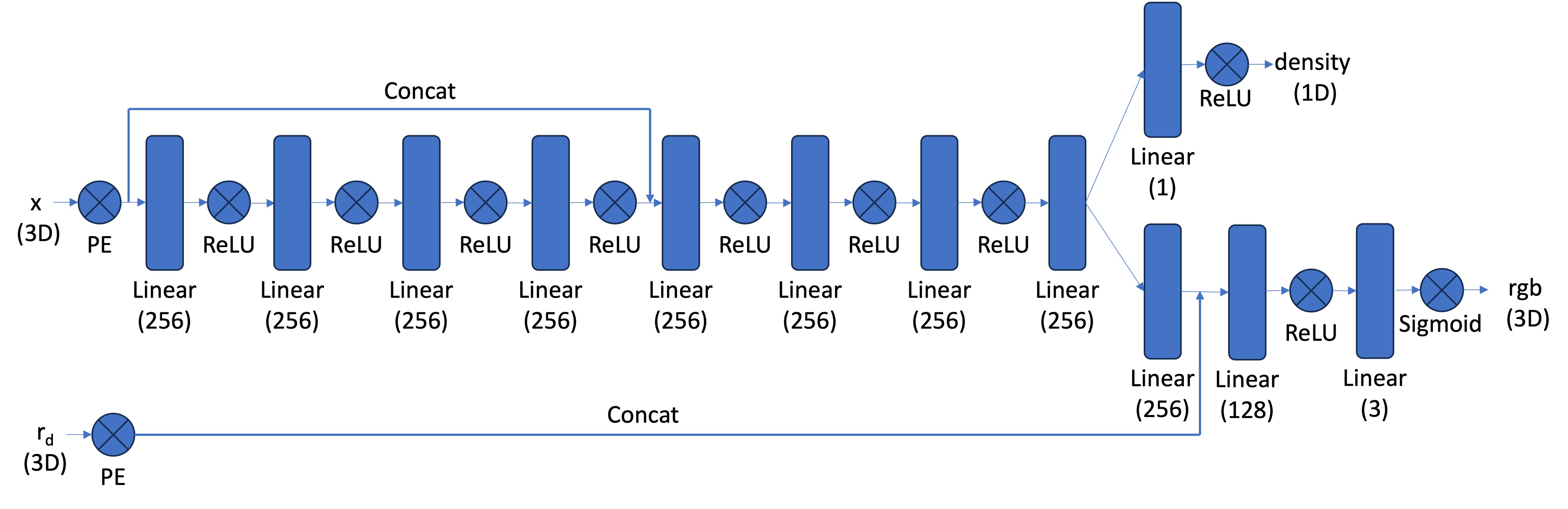
Part 2.4: Neural Radiance Field
Similarly, we will also implement the NeRF model that we saw in Part 1. However, we will add some more layers to make it compatible for 3D objects so we can produce the nice view at the end.
An image of the network we implemented can be seen below:
 {width=“90%”, fig-align=“center”}
For this part, we basically replicate the code we have seen in Part 1, but make it slightly more complicated as the diagram shown for this problem is relatively more complicated than the one shown in Part 1.
Part 2.5: Volume Rendering
Finally, we will implement the equation that resembles how colors on the rays work, using the following approximate equation:
\[\begin{align} \hat{C}(\mathbf{r})=\sum_{i=1}^N T_i\left(1-\exp \left(-\sigma_i \delta_i\right)\right) \mathbf{c}_i, \text { where } T_i=\exp \left(-\sum_{j=1}^{i-1} \sigma_j \delta_j\right) \end{align}\]
We also pass the following test cases, which seems to be a good sign that our implementation is correct:
torch.manual_seed(42)
sigmas = torch.rand((10, 64, 1))
rgbs = torch.rand((10, 64, 3))
step_size = (6.0 - 2.0) / 64
rendered_colors = volrend(sigmas, rgbs, step_size)

correct = torch.tensor([
    [0.5006, 0.3728, 0.4728],
    [0.4322, 0.3559, 0.4134],
    [0.4027, 0.4394, 0.4610],
    [0.4514, 0.3829, 0.4196],
    [0.4002, 0.4599, 0.4103],
    [0.4471, 0.4044, 0.4069],
    [0.4285, 0.4072, 0.3777],
    [0.4152, 0.4190, 0.4361],
    [0.4051, 0.3651, 0.3969],
    [0.3253, 0.3587, 0.4215]
  ])
assert torch.allclose(rendered_colors, correct, rtol=1e-4, atol=1e-4)
To implement this part, we have followed the hint and used cumprod to get the probability of light stopping at a certain point as instructed in lecture. Similarly, we also implemented a training loop that will help us train our model against the lego dataset before we actually play around with the real dataset with my stitch.
A visualization of the rays being sampled at a timestep can be seen below:
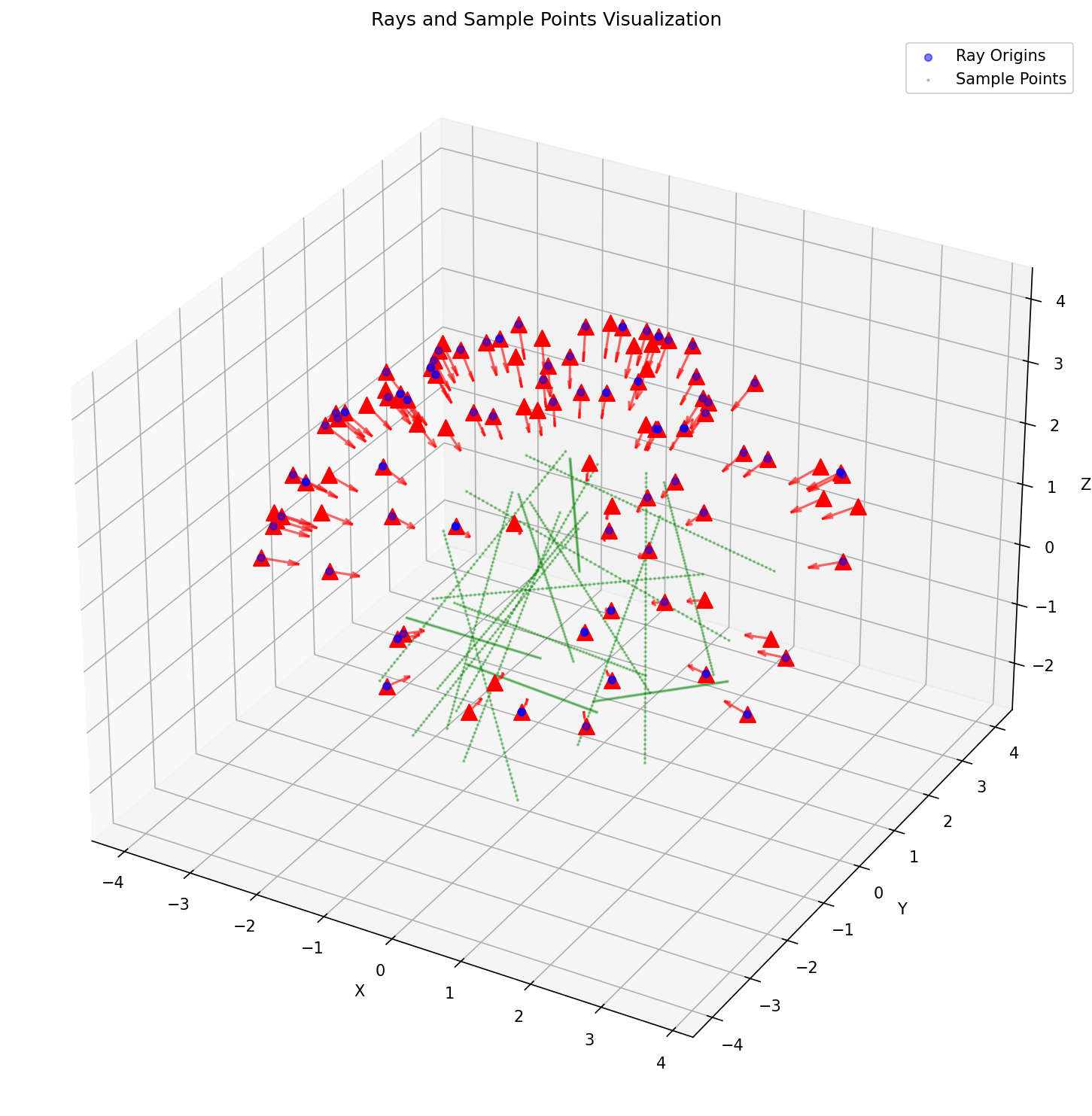 {width=“80%”, fig-align=“center”}
We will also see how the PSNR diagrams and during the training process, what the rendered images from a particular angle will look like:
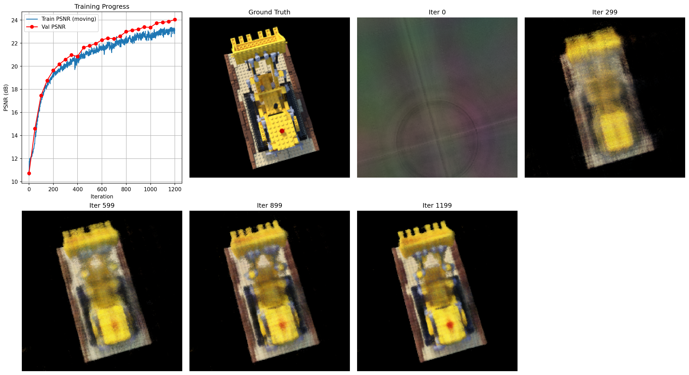
At step 0, we see basically nothing. You cannot tell what it actually is. However, we see a major improvement at step 299, and as we increase the number of steps in training, it looks more like the ground truth. Unfortunately, we are still a very long way until it is smooth and has edges like the ground truth.
However, we have generated a somewhat successful spherical view of the lego, which is close to what is shown in the guidelines:
Part 2.6: Training with your own data
Finally, we will get to our own data. Unfortunately, the actual result isn’t what I anticipated it to be, but I tried my best to get the progress I can get.
The following is the PSNR curve, which we trained for 50,000 iterations:
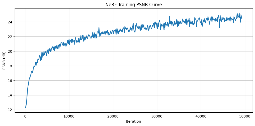 {width=“80%”, fig-align=“center”}
And the loss curve for reference:
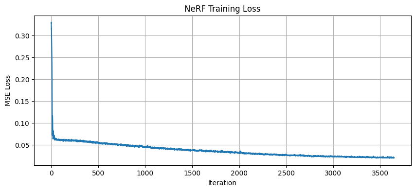 {width=“80%”, fig-align=“center”}
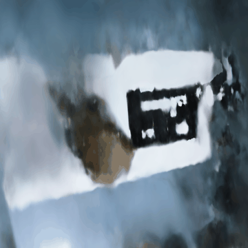
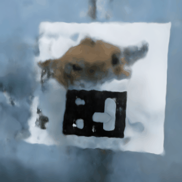
The following are some rendered images that we saw as we were training:
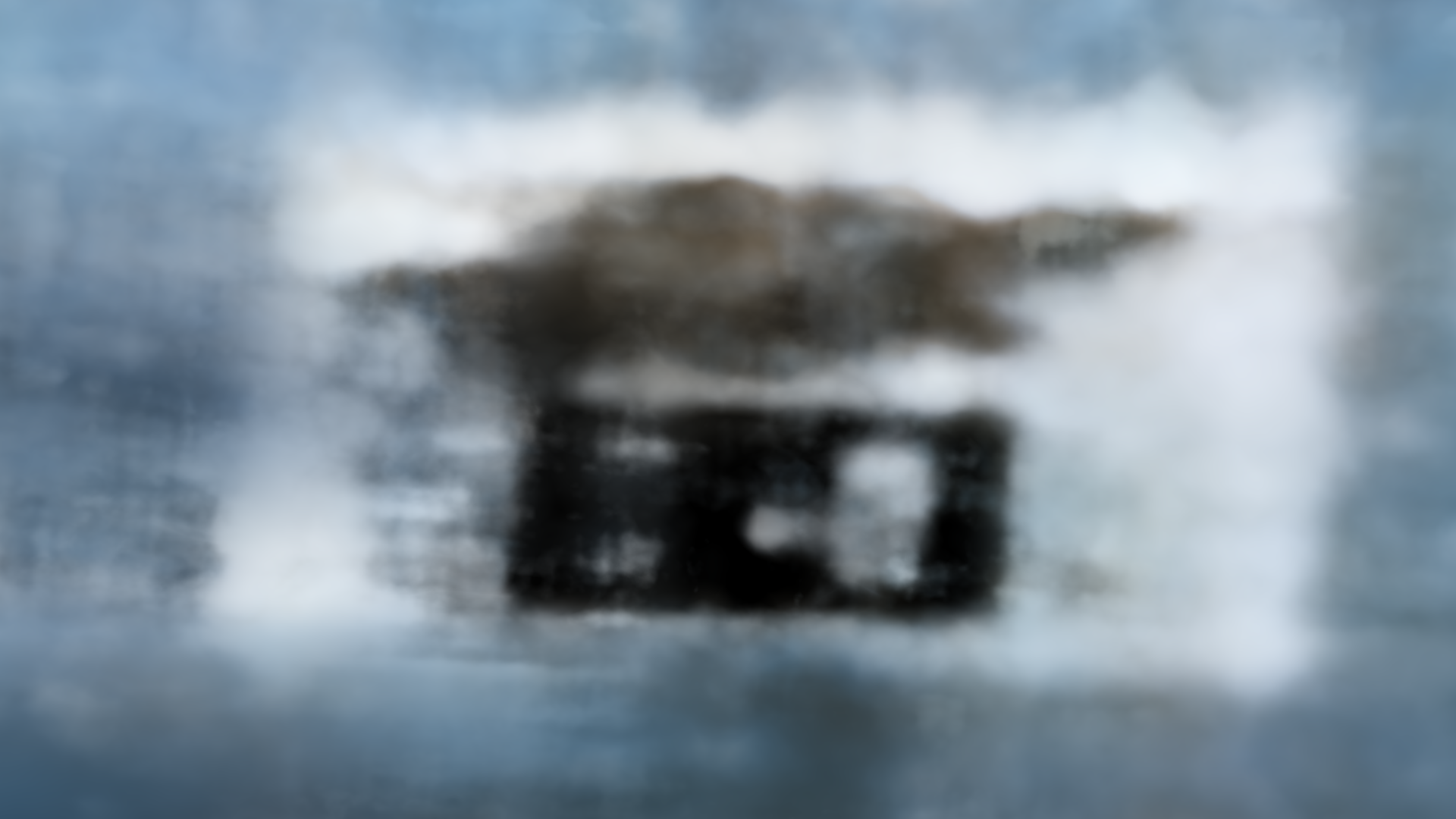
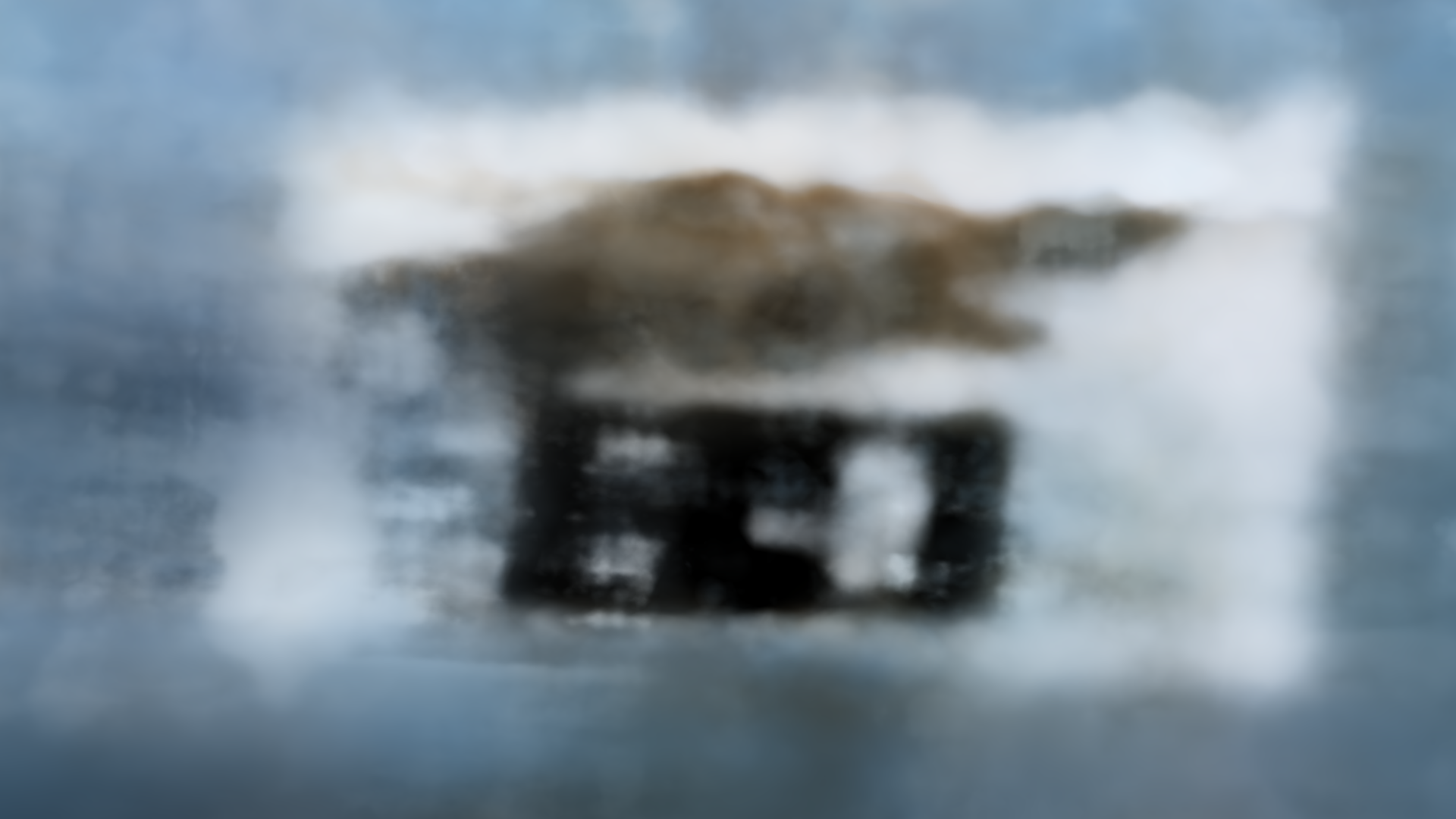
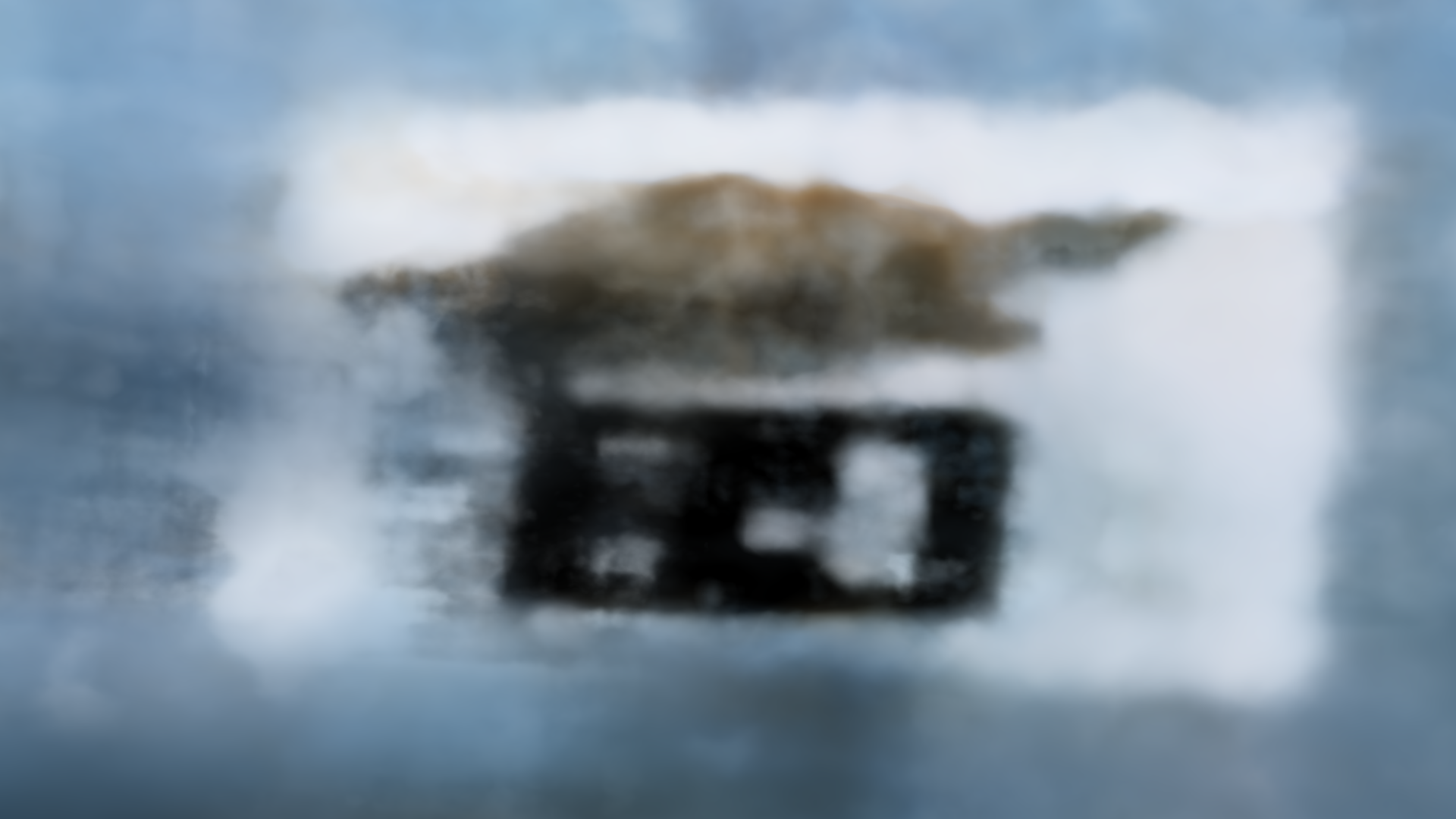
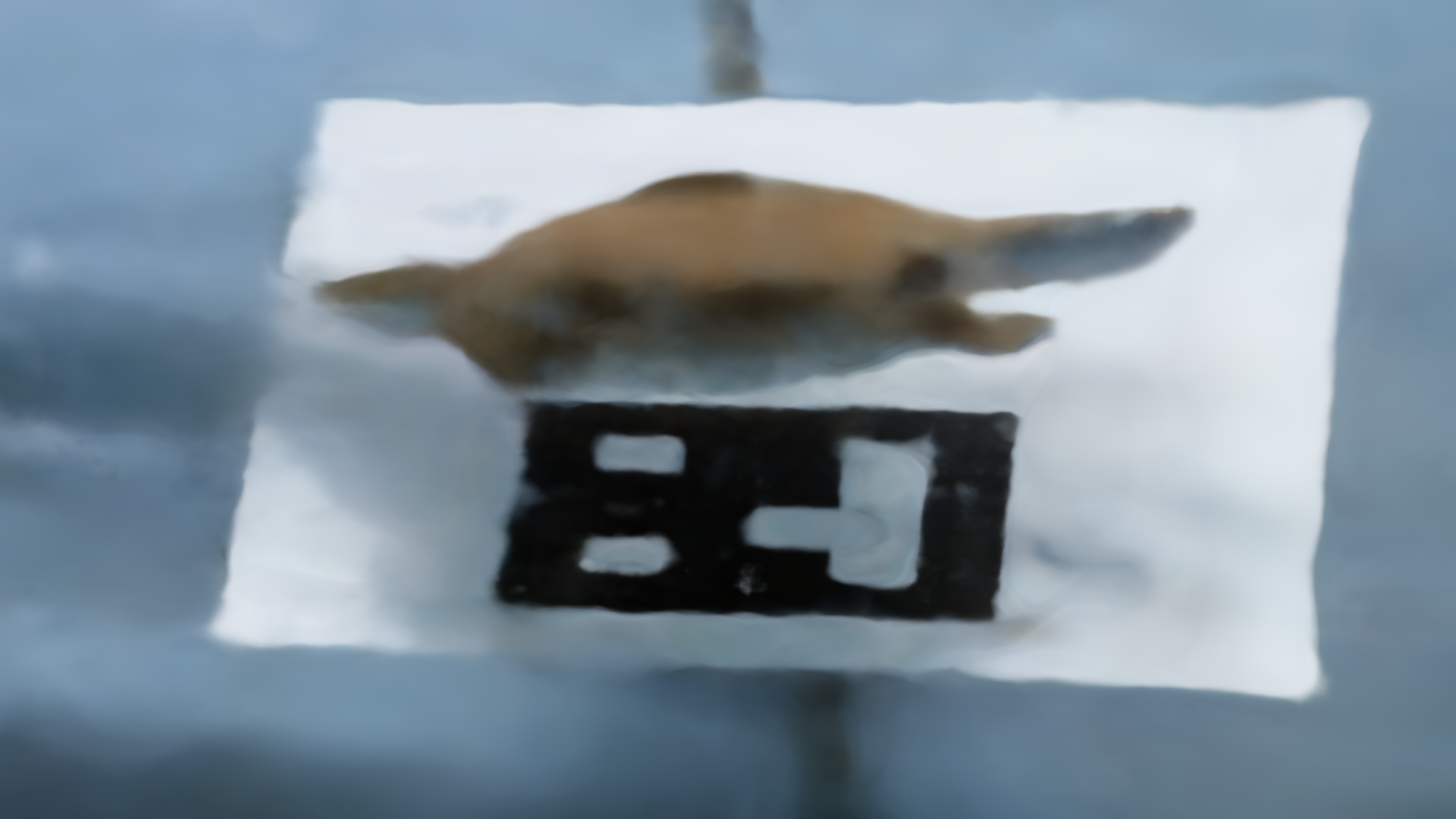
We see that as we are increasing the number of iterations, the stitch case is becoming more apparent from nothing, which is interesting. Some patterns are similar to what we saw in the lego scene. However, unfortunately, it’s not as clear as we had wanted.
Now, for the final GIFs, though they are definitely far from perfect:
We will have two GIFs for reference, where in each one you can see the stitch case in some scenes:
Compared to the lego scene, as mentioned in the hint, we have adjusted the near and far parameters. Since my camera was much closer to the object than what was presented in the paper, we have adjusted to what the hint was suggesting: near = 0.02 and far = 0.5. Everything else was very similar, as we believed it should follow the same correct code that generated the lego scene correctly.