CS 180 Project 3: [Auto]Stitching Photo Mosaics
In this project, I will present a set of source photographs, carefully identify key correspondences between them, and then apply image warping techniques to align the photos before compositing them into a seamless final result.
Part A: Image Warping and Mosaicing
In this part of the project, we will explore how image mosaicing works and see how it can transform pairs or even triples of images by stitching them together into a smooth and visually appealing composite.
Shoot the Pictures
There are many different kinds of transformations that we can apply to images, such as translation, rotation, and affine transformations.
In this project, we will skip the simpler ones (or treat them as special cases) and instead focus on the more general and powerful perspective or projective transformation.
In some sense, projective transformations extend affine transformations by introducing the ability to model perspective effects. They can be thought of as projective warps, and they have the following properties:
- The origin does not necessarily map to the origin.
- Lines map to lines.
- Parallel lines do not necessarily remain parallel.
- Ratios of distances are not preserved.
- They are closed under composition.
- They can be interpreted as modeling a change of basis in projective space.
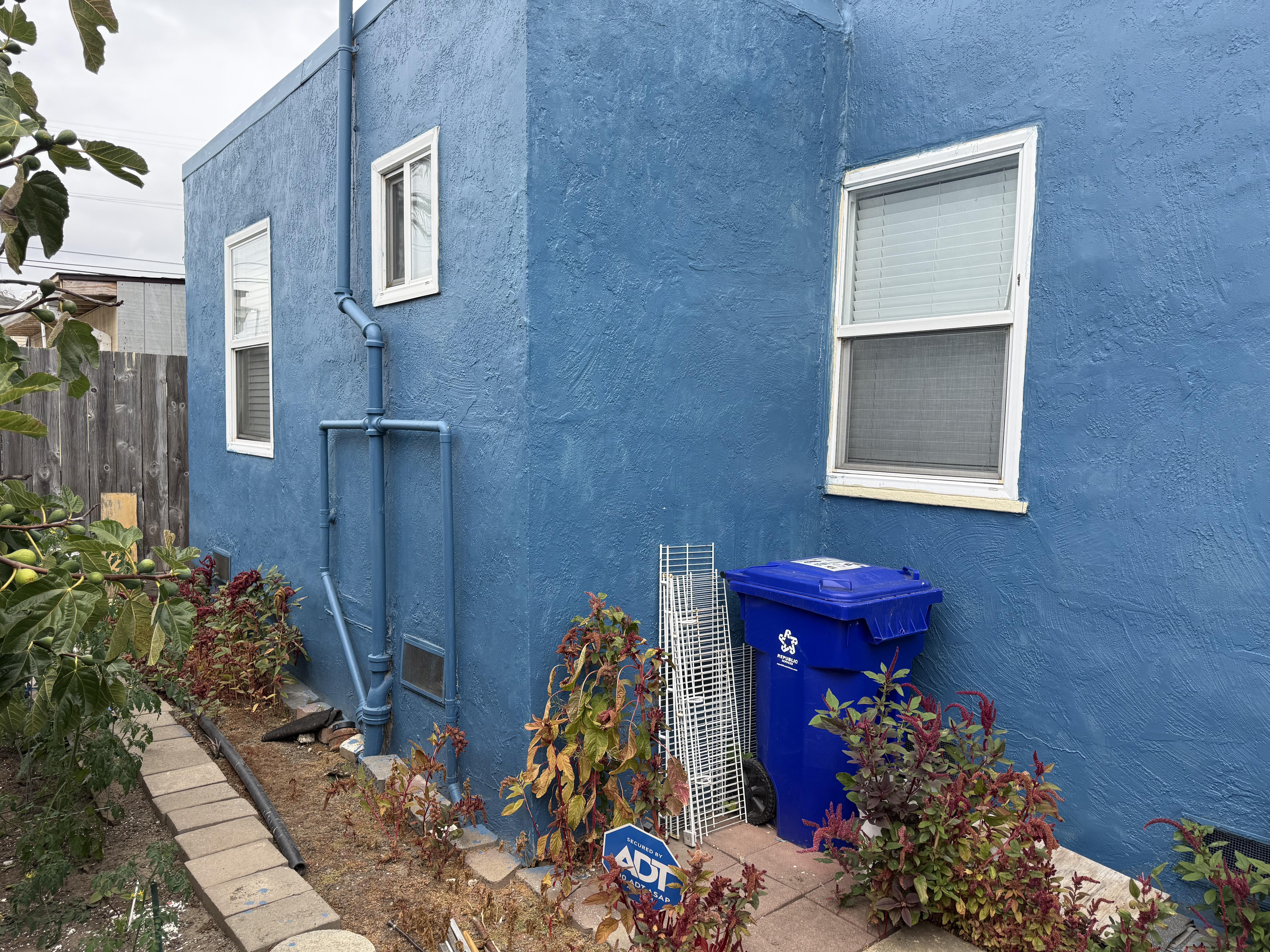
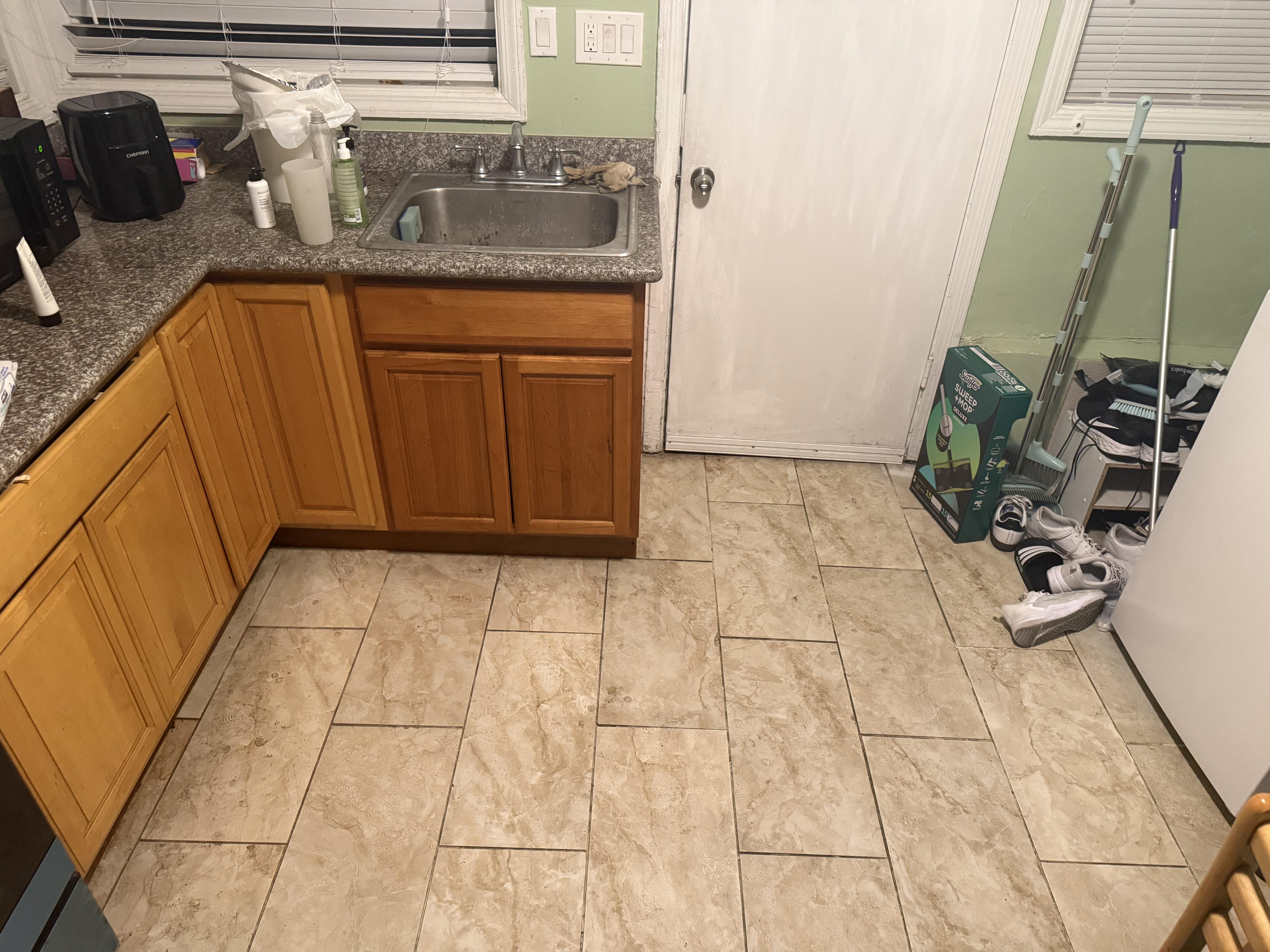
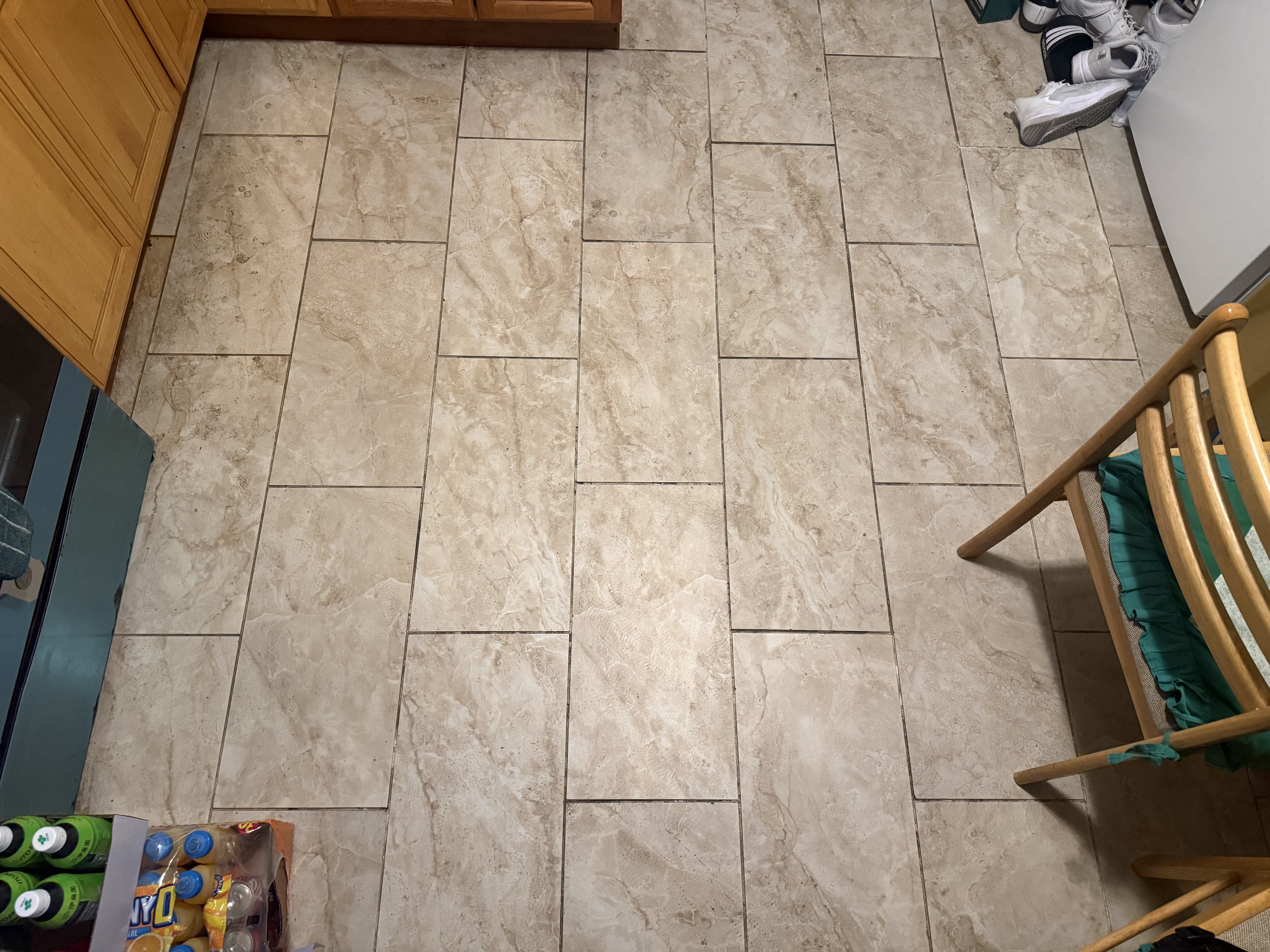
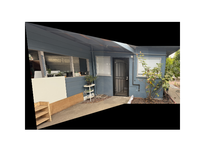
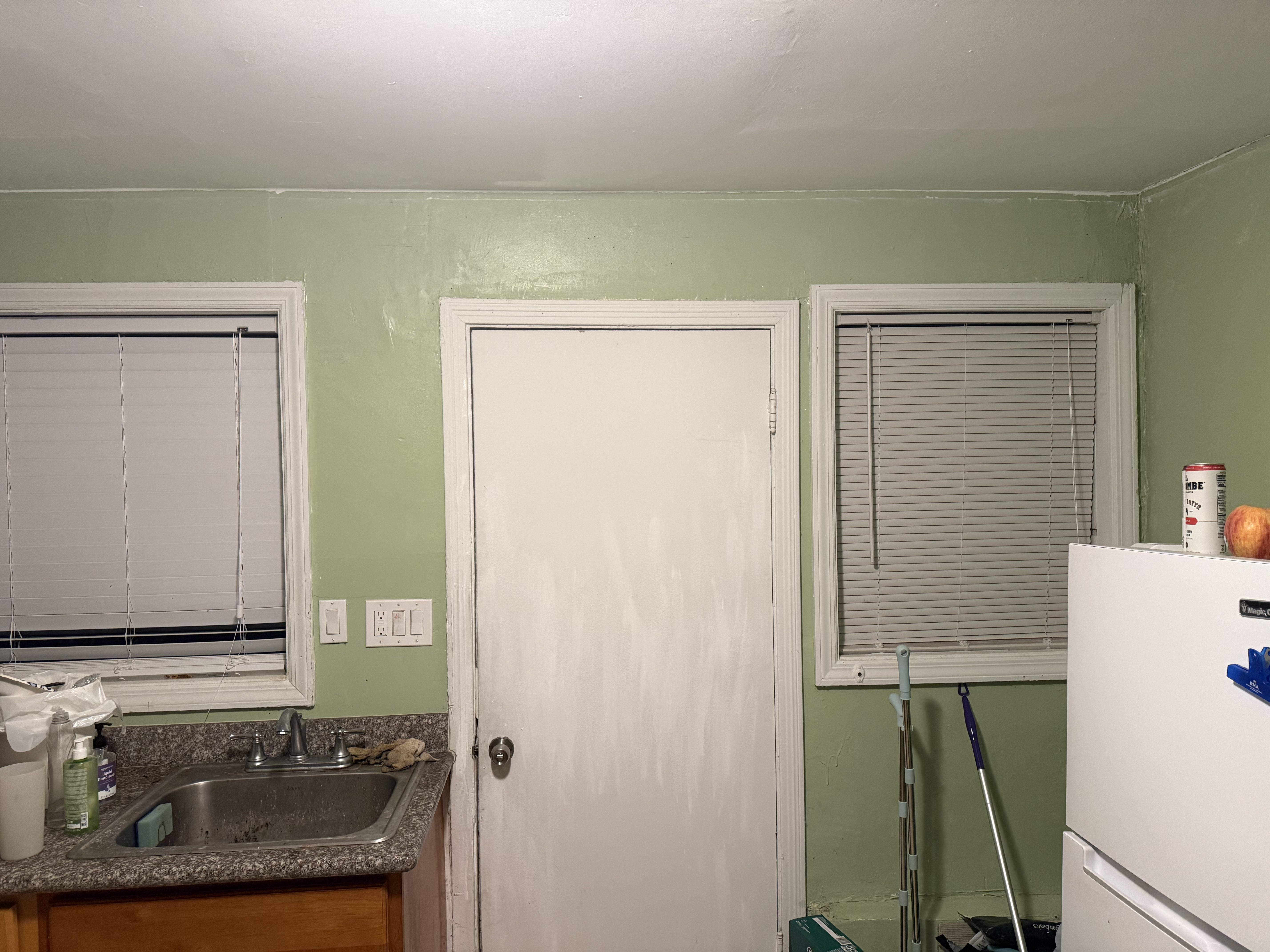
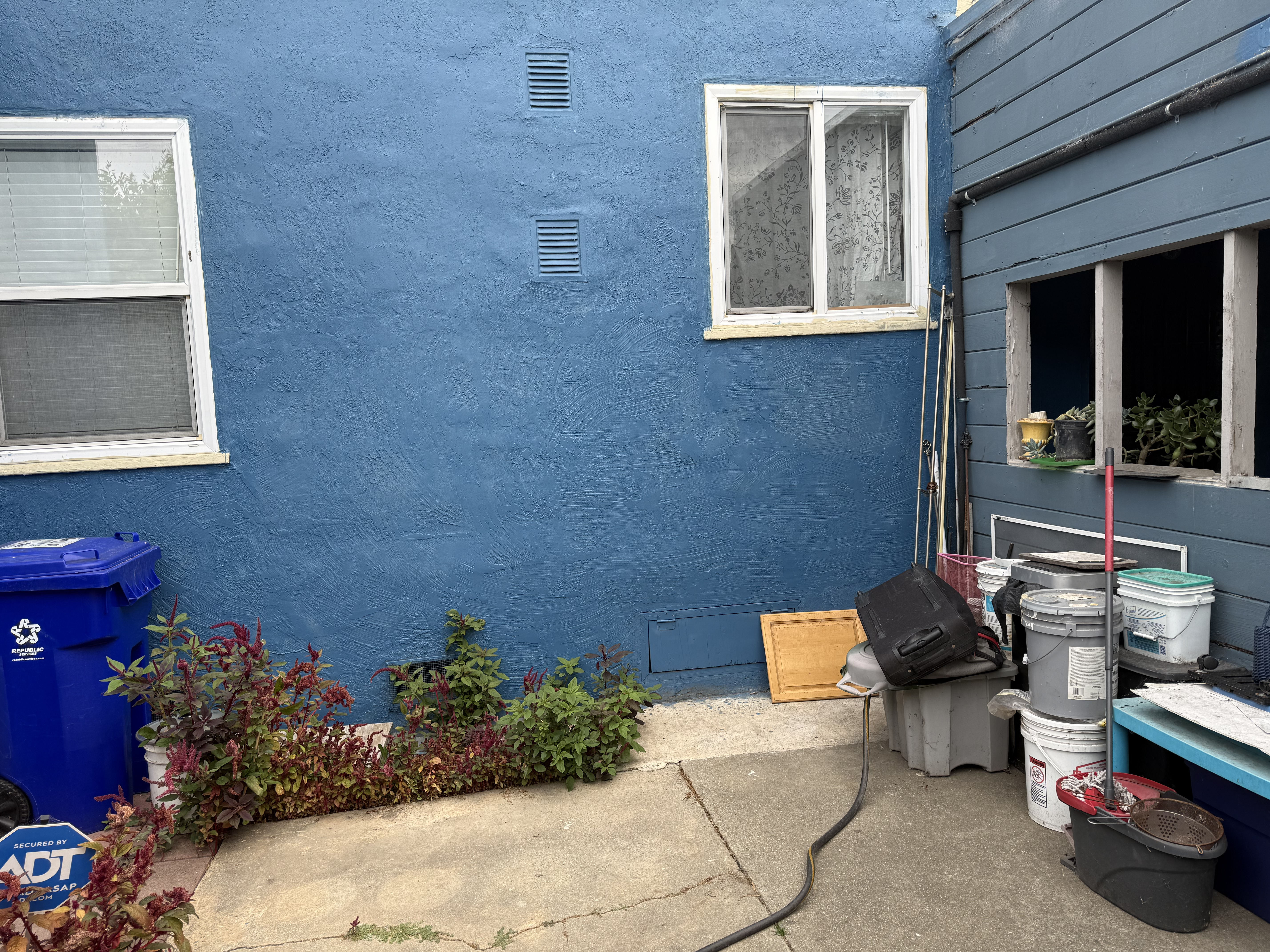
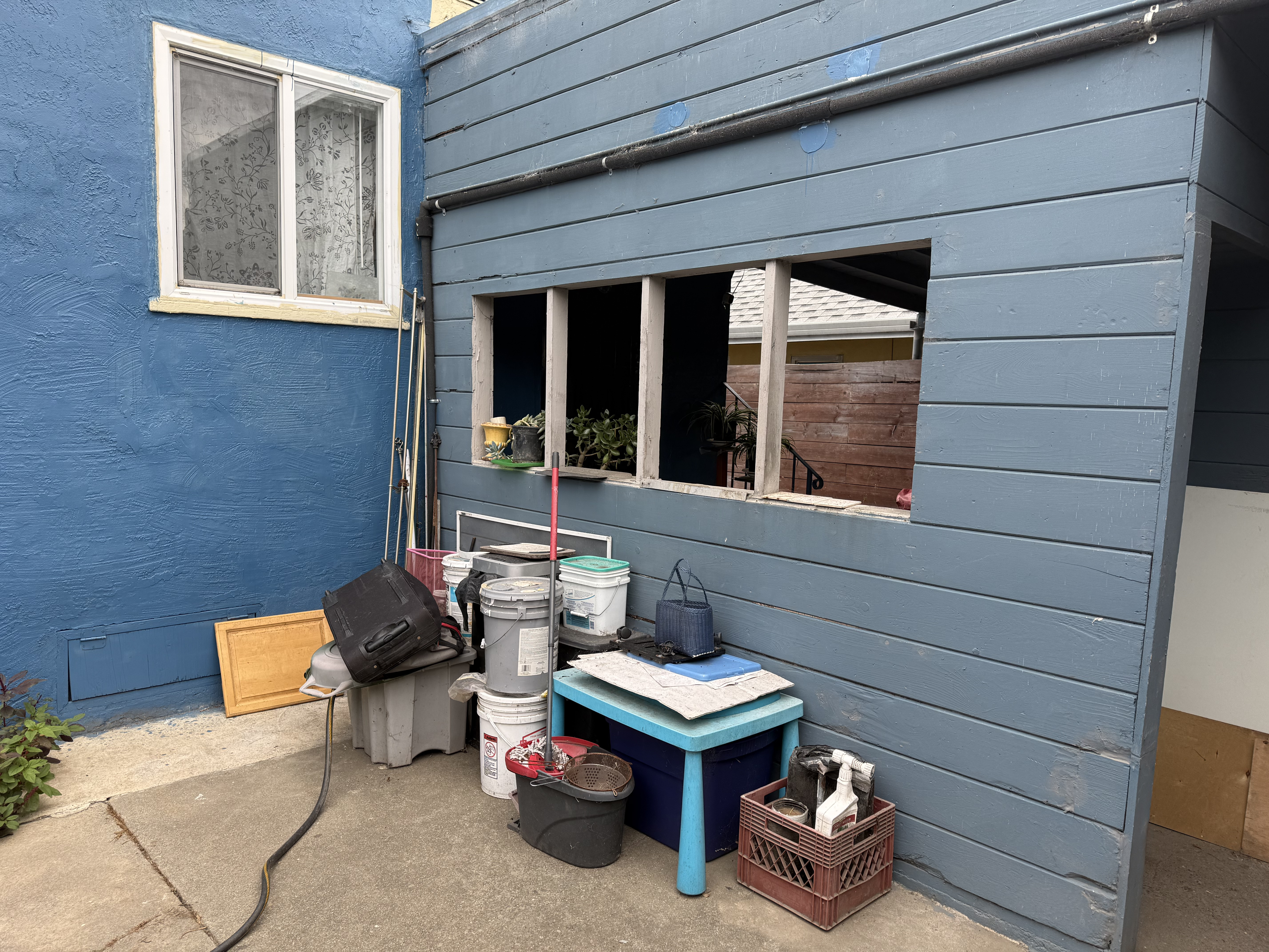
The following pairs of pictures were taken in my neighborhood, around my house:
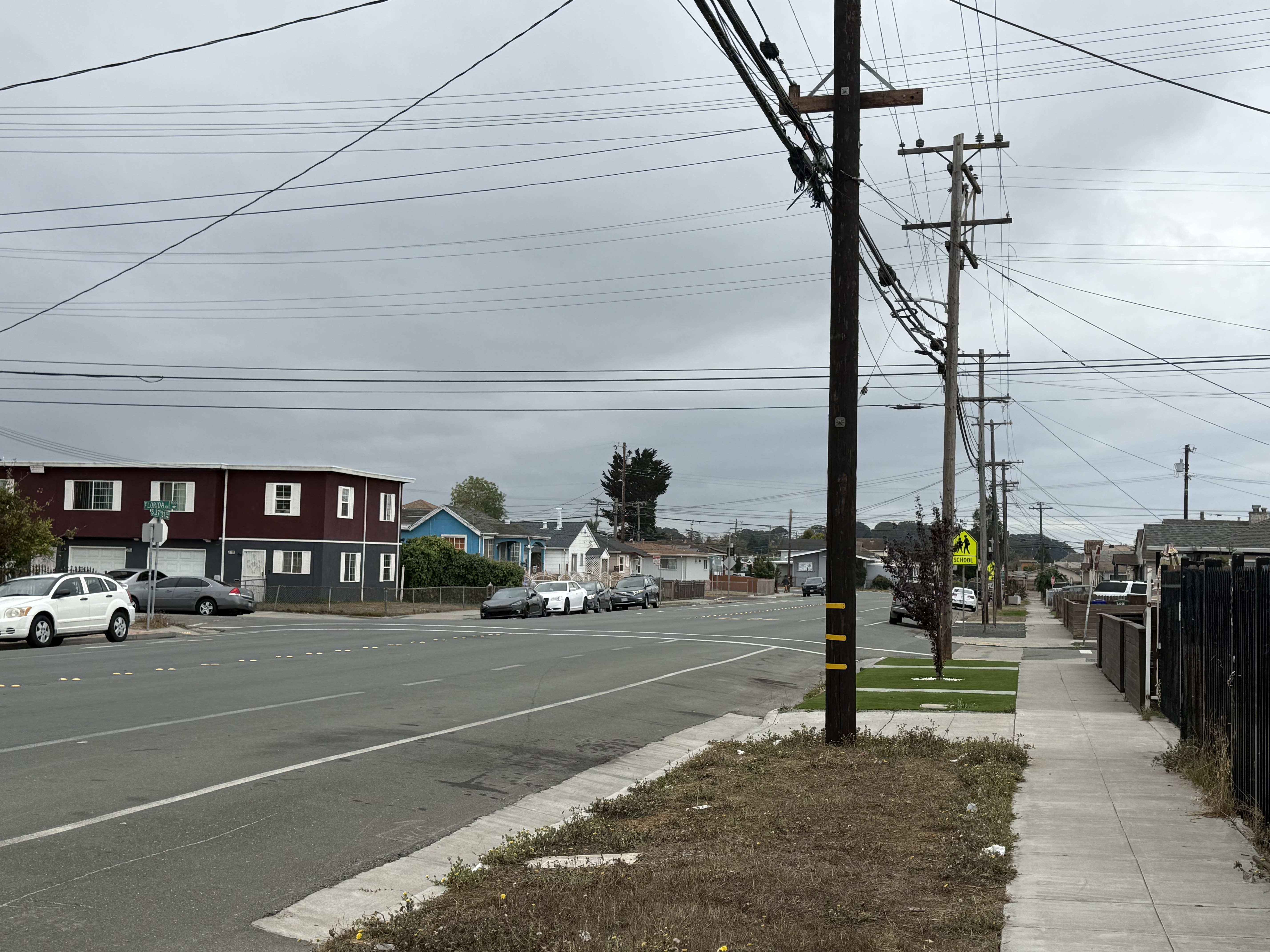
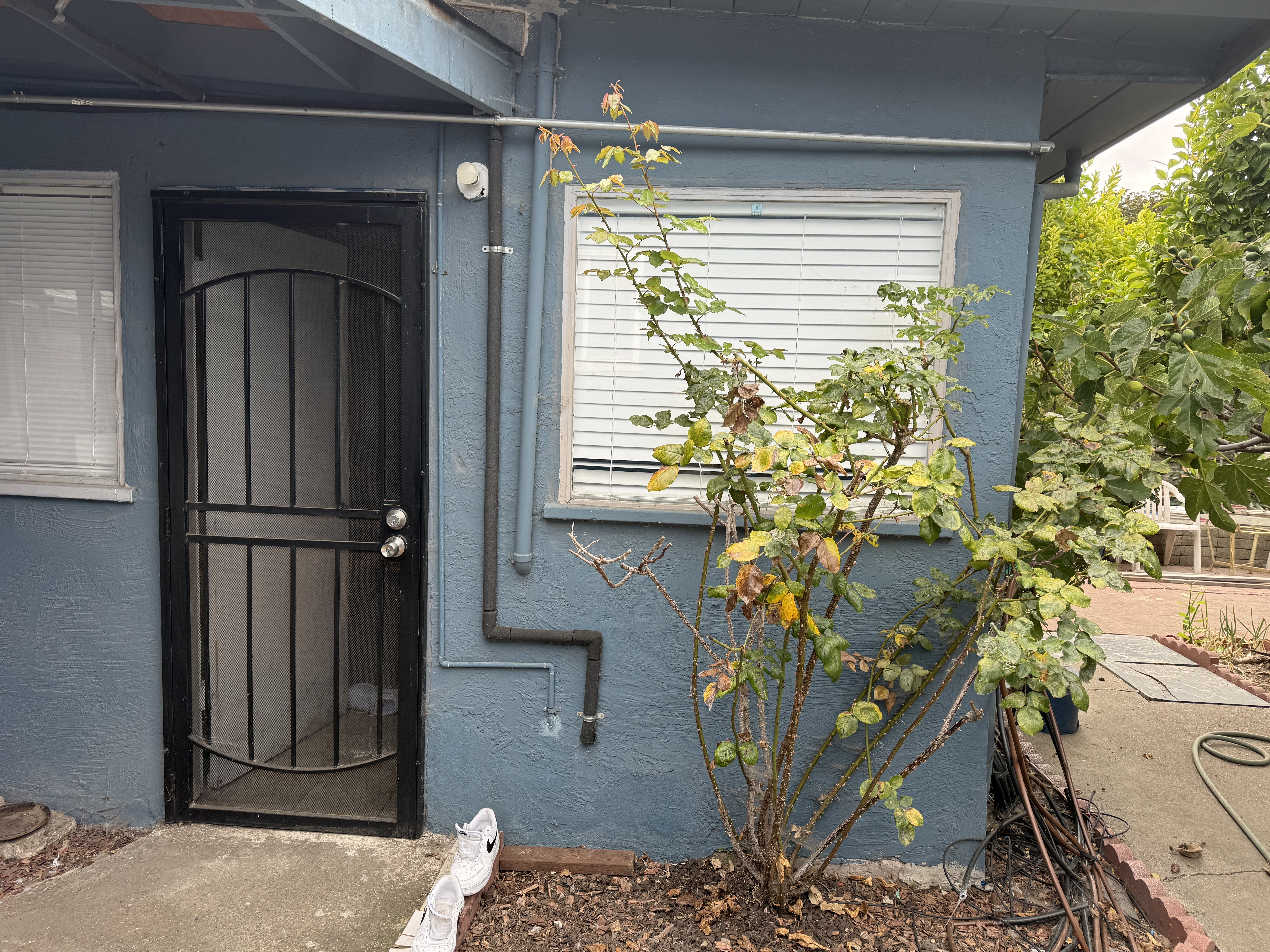
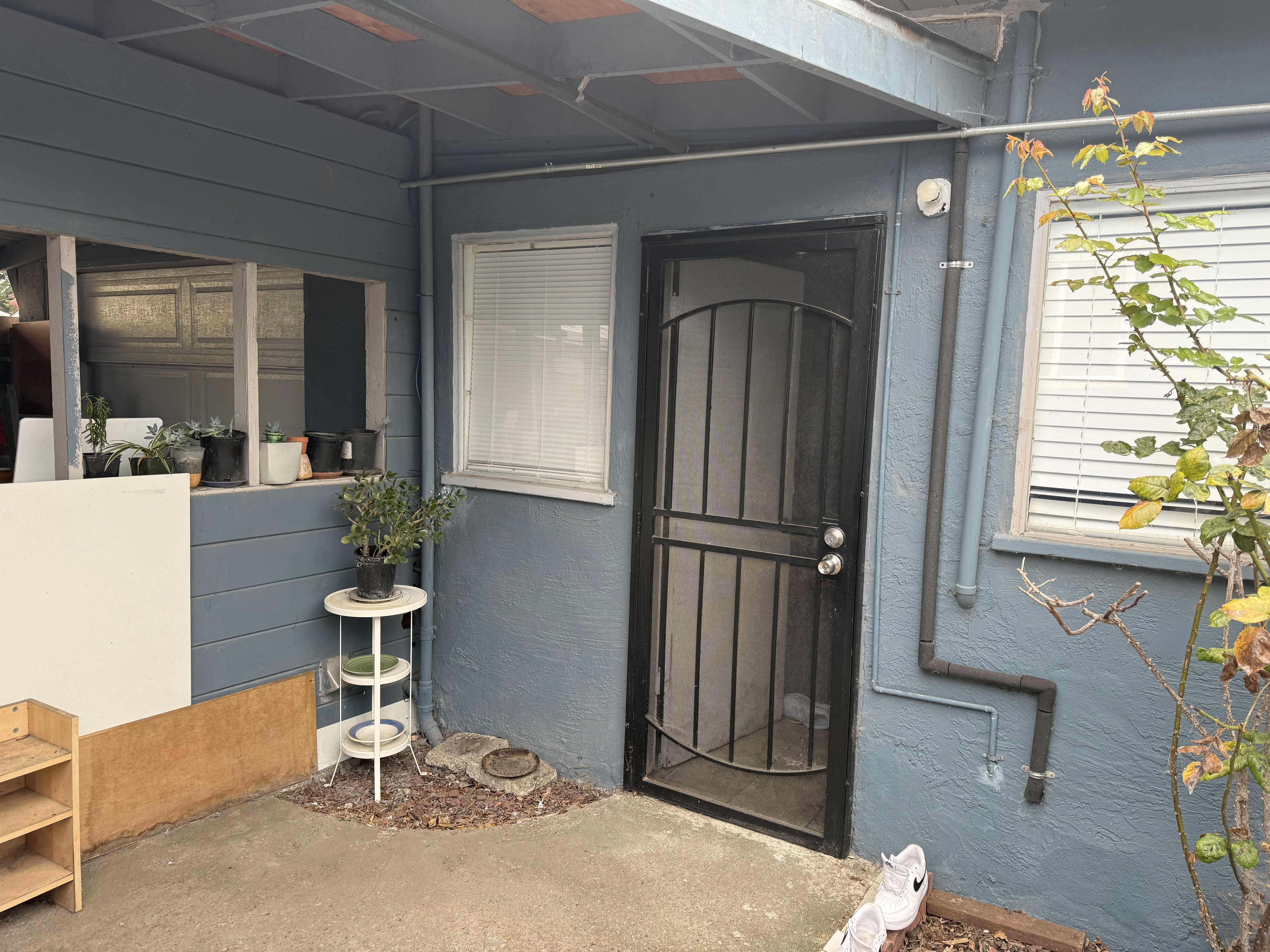
As seen in the pictures, the center of perspective (where the camera lens of my iPhone is located) remains fixed. What changes is the rotation of the camera relative to the scene, which results in a projective transformation.
Of course, since the camera was handheld, the alignment is not perfectly precise. However, it should still be clear why this situation can be modeled as a projective transformation. As we will see later, these two pictures can be merged together into a single, seamless image.
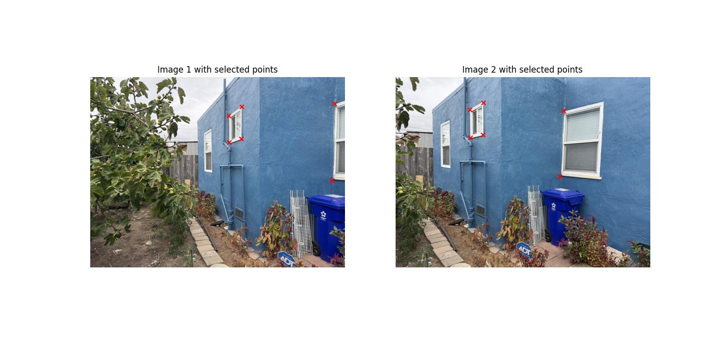
Recover Homographies
To stitch the images together smoothly, we will implement a homography function, which allows us to recover the transformation between the left image and the right image.
After solving for this relationship, we obtain a matrix \(H\) by setting up and solving a system of equations based on points that we select and believe to correspond to the same locations in both images.
Once \(H\) is computed, we can use it to project one image into the coordinate system of the other, effectively aligning them so that they appear to lie on the same “plane” or “face.”
For example, for the pair of house images shown above, we compute the following homography matrix \(H\):
\[ H = \begin{bmatrix} -0.00038728 & -0.00002103 & 0.95231 \\ -0.00006998 & -0.00032202 & 0.30514 \\ -0.00000003677 & -0.00000000327 & -0.00016545 \end{bmatrix} \]
This matrix was computed by solving a linear system derived from 6 pairs of corresponding points.
Each pair of points contributes two equations, giving us a total of 12 equations in the 9 unknowns of \(H\) (up to scale).
The stacked system of equations has the form:
\[ A \mathbf{h} = 0 \]
where \(\mathbf{h}\) is the vectorized form of the homography matrix entries.
To compute the homography matrix \(H\), we set up a system of linear equations based on point correspondences.
For each pair \((x, y) \leftrightarrow (x', y')\), the following two equations are added:
\[ \begin{bmatrix} x & y & 1 & 0 & 0 & 0 & -x'x & -x'y & -x' \\ 0 & 0 & 0 & x & y & 1 & -y'x & -y'y & -y' \end{bmatrix} \begin{bmatrix} h_{11} \\ h_{12} \\ h_{13} \\ h_{21} \\ h_{22} \\ h_{23} \\ h_{31} \\ h_{32} \\ h_{33} \end{bmatrix} = 0 \]
Stacking all \(n\) correspondences produces the matrix equation
\[ A \mathbf{h} = 0 \]
where \(A \in \mathbb{R}^{2n \times 9}\) and \(\mathbf{h}\) is the 9-vector formed by vectorizing \(H\).
For our 6 pairs of points, the explicit \(A\) matrix is:
\[ A = \begin{bmatrix} 2884.36 & 1079.34 & 1 & 0 & 0 & 0 & -1988184.04 & -743983.92 & -689.30 \\ 0 & 0 & 0 & 2884.36 & 1079.34 & 1 & -2534882.22 & -948559.87 & -878.84 \\ 3979.87 & 969.74 & 1 & 0 & 0 & 0 & -7684924.23 & -1872506.84 & -1930.95 \\ 0 & 0 & 0 & 3979.87 & 969.74 & 1 & -3611233.71 & -879912.36 & -907.37 \\ 2814.29 & 3575.21 & 1 & 0 & 0 & 0 & -2094245.50 & -2660478.37 & -744.15 \\ 0 & 0 & 0 & 2814.29 & 3575.21 & 1 & -10448251.70 & -13273204.00 & -3712.57 \\ 3788.44 & 3848.38 & 1 & 0 & 0 & 0 & -7127880.47 & -7240670.25 & -1881.48 \\ 0 & 0 & 0 & 3788.44 & 3848.38 & 1 & -14317456.80 & -14544012.60 & -3779.25 \\ 2770.92 & 1001.85 & 1 & 0 & 0 & 0 & -1420188.23 & -513481.40 & -512.53 \\ 0 & 0 & 0 & 2770.92 & 1001.85 & 1 & -2177778.95 & -787394.91 & -785.94 \\ 2727.46 & 2249.37 & 1 & 0 & 0 & 0 & -1558763.97 & -1285532.42 & -571.51 \\ 0 & 0 & 0 & 2727.46 & 2249.37 & 1 & -6113241.06 & -5041667.46 & -2241.37 \end{bmatrix} \]
The unknown vector is
\[ \mathbf{h} = \begin{bmatrix} h_{11} & h_{12} & h_{13} & h_{21} & h_{22} & h_{23} & h_{31} & h_{32} & h_{33} \end{bmatrix}^T \]
We solve this homogeneous system using Least Squares as we have an overdetermined system (which is done intentionally to increase the accuracy of the matrix).
Finally, we reshape \(\mathbf{h}\) into the \(3 \times 3\) matrix \(H\) (defined up to scale), giving the homography.
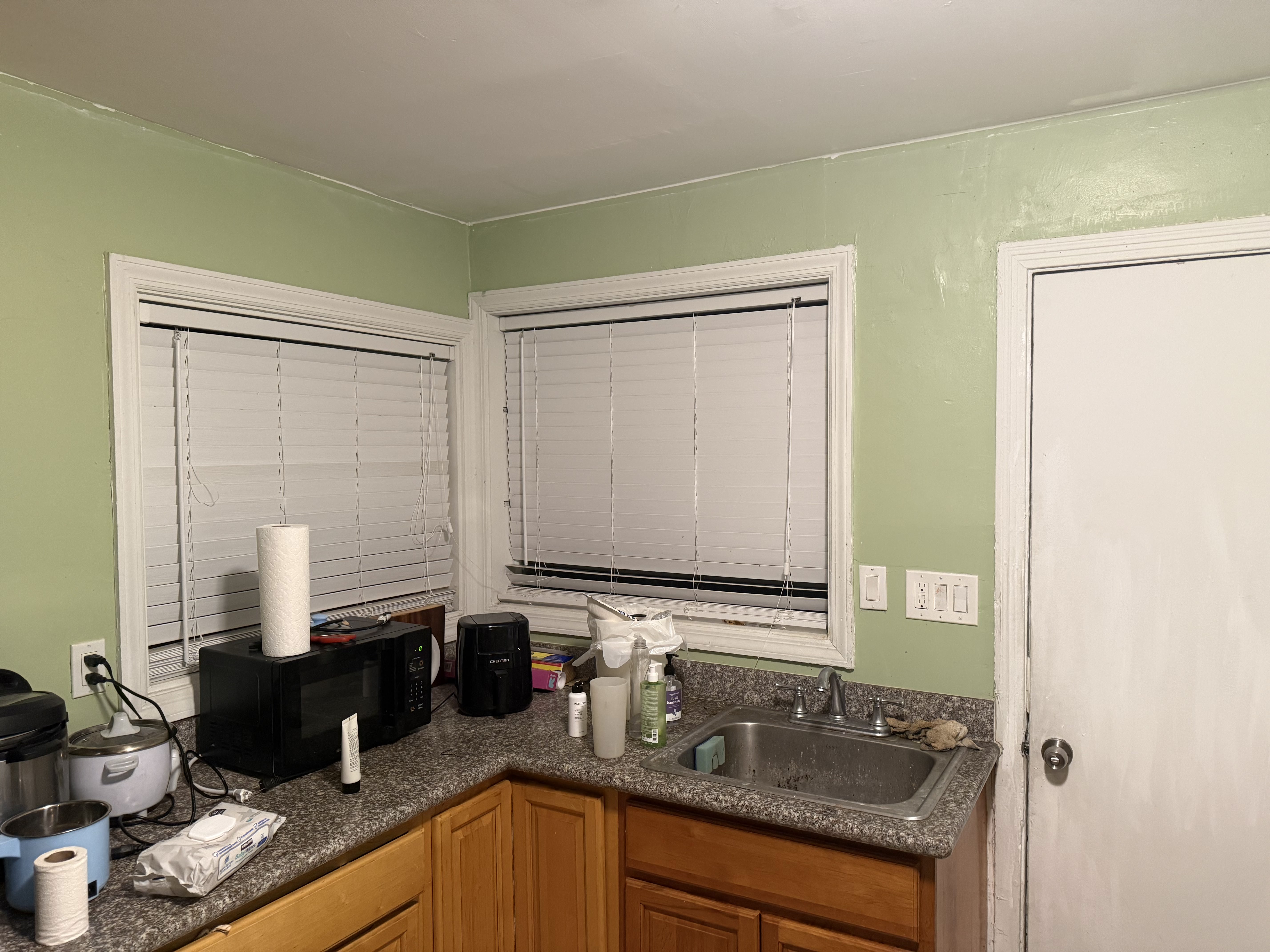
Similarly, for this pair of images:
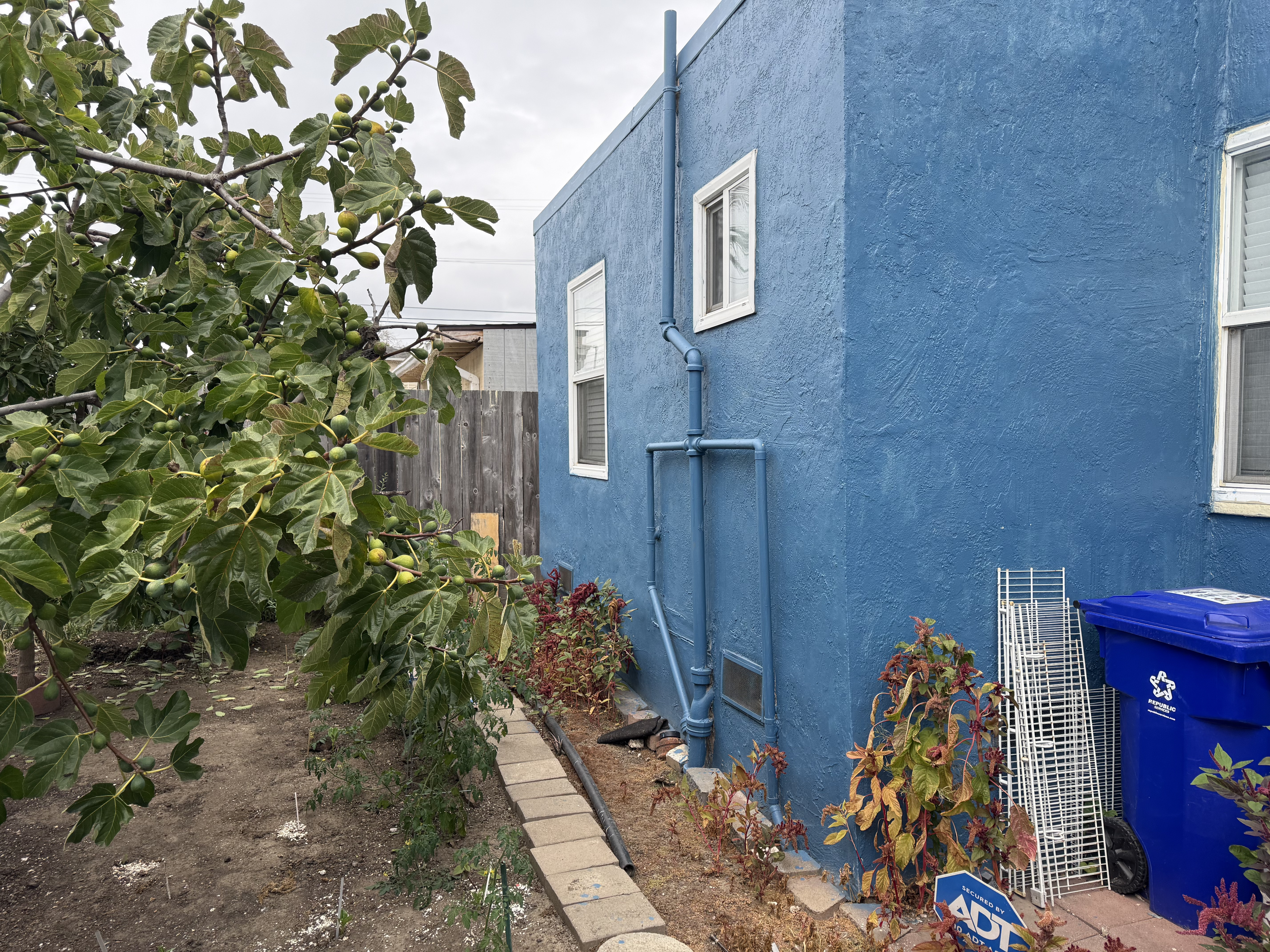
We selected 6 pairs of corresponding points and computed the following homography matrix \(H\):
\[ H = \begin{bmatrix} -0.00033191 & 0.00001756 & -0.97032 \\ 0.00009397 & -0.00045974 & -0.24181 \\ 0.00000003948 & 0.00000000566 & -0.00055601 \end{bmatrix} \]
The system of equations used to solve for \(H\) is:
\[ A \mathbf{h} = 0, \]
where each point correspondence \((x, y) \leftrightarrow (x', y')\) contributes two rows to \(A\).
For the 6 pairs of points, the matrix \(A\) in full decimal form is:
\[ A = \begin{bmatrix} 3778.80 & 774.16 & 1 & 0 & 0 & 0 & -20759760.00 & -4253028.21 & -5493.74 \\ 0 & 0 & 0 & 3778.80 & 774.16 & 1 & -2277016.13 & -466489.66 & -602.58 \\ 3678.41 & 2224.31 & 1 & 0 & 0 & 0 & -19883545.80 & -12023465.00 & -5405.48 \\ 0 & 0 & 0 & 3678.41 & 2224.31 & 1 & -8480479.35 & -5128096.77 & -2305.48 \\ 1672.26 & 747.14 & 1 & 0 & 0 & 0 & -5208653.58 & -2327134.14 & -3114.74 \\ 0 & 0 & 0 & 1672.26 & 747.14 & 1 & -1464282.59 & -654215.52 & -875.63 \\ 1668.11 & 1391.81 & 1 & 0 & 0 & 0 & -5188328.31 & -4328943.74 & -3110.31 \\ 0 & 0 & 0 & 1668.11 & 1391.81 & 1 & -2499986.68 & -2085893.77 & -1498.70 \\ 1963.47 & 569.95 & 1 & 0 & 0 & 0 & -6658797.55 & -1932881.63 & -3391.35 \\ 0 & 0 & 0 & 1963.47 & 569.95 & 1 & -1323781.52 & -384260.52 & -674.21 \\ 1968.38 & 1311.65 & 1 & 0 & 0 & 0 & -6685178.87 & -4454754.64 & -3396.29 \\ 0 & 0 & 0 & 1968.38 & 1311.65 & 1 & -2777887.22 & -1851080.76 & -1411.26 \end{bmatrix} \]
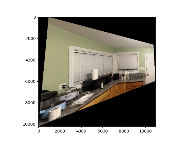
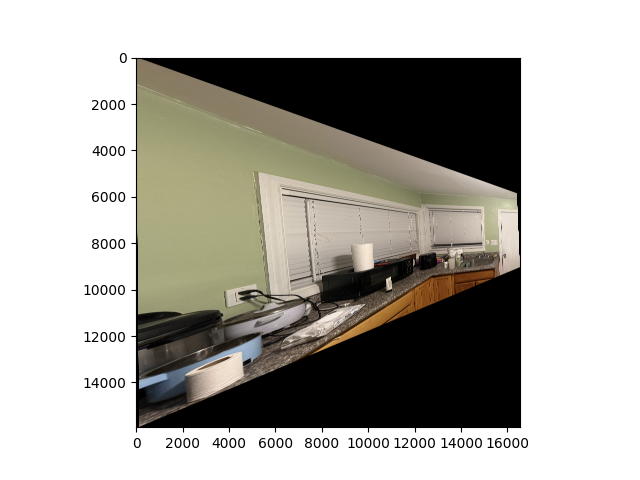
Warp the Images
Now we will actually warp the images, since we have recovered the homography matrix previously.
Specifically, there are two main ways to map the indices from the original image to the warped image:
Nearest Neighbor Interpolation
For each pixel in the output canvas (the warped version of the image), we want to determine its corresponding RGB values from the original image.
- If the mapped coordinates are integers, we can directly perform a one-to-one mapping.
- However, most of the time the mapped coordinates are not integers. In this case, the nearest neighbor method chooses the pixel from the original image that is closest to the mapped coordinate.
This method is simple and fast. While it is not perfect and can produce blocky artifacts, the effect becomes less noticeable if the image has high resolution.
- If the mapped coordinates are integers, we can directly perform a one-to-one mapping.
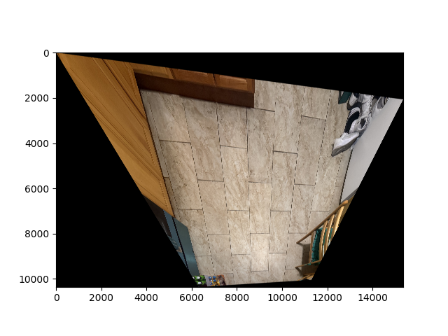
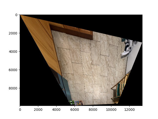
The following images are warped using the bilinear interpolation method:
Bilinear Interpolation
The nearest neighbor method has the disadvantage of producing sharp edges and blocky artifacts, especially when the image is scaled or rotated.
Bilinear interpolation improves on this by taking a weighted average of the four nearest pixels in the original image.- This produces smoother transitions in the warped image and generally looks more natural.
- Although it is slightly more computationally expensive than nearest neighbor interpolation, it is usually preferred when visual quality is important.
- This produces smoother transitions in the warped image and generally looks more natural.
The following images are warped using the bilinear interpolation method:
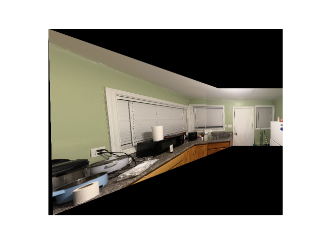
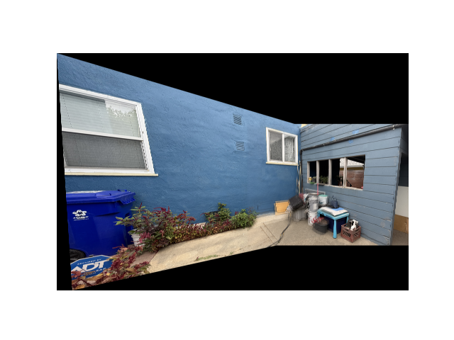
Blend the Images into a Mosaic
For the final step, we will be blending several images that have the same center of perspetive into a mosaic, which is pretty cool! Soemthing that I always have been fascinated abotu and never thought could be done with computer science.
To reduce the edge effects we use alpha masking here so everything would look nice.
We went through the following procedure:
Step 1: Determine the Canvas Size
We first calculate the canvas size to ensure that all images fit entirely after warping.
Step 2: Place the Warped Images on the Canvas
- The first image is placed directly at the top-left corner of the canvas.
- The second (or subsequent) image is shifted according to the coordinates of its selected points after warping.
Step 3: Create Alpha Masks for Smooth Blending
To avoid harsh boundaries, we compute alpha masks with a linear falloff from the center to the edges (using make_alpha_mask).
These masks ensure that pixel contributions fade smoothly near the edges, reducing visible seams.
Step 4: Apply Masks and Ignore Black Pixels
We multiply each image by its alpha mask while ignoring black pixels (apply_mask_with_black_ignore).
This isolates valid image regions and prevents empty pixels from influencing the blending.
Step 5: Weighted Averaging for Blending
Weighted contributions from each image are combined to produce the final blended mosaic.
This procedure avoids overwriting pixels and blends overlapping regions proportionally to their alpha values.
Step 6: Crop to Nonzero Regions
After blending, we crop the mosaic to remove empty borders (using crop_to_bounds).
The result is a final mosaic with smooth transitions and minimal edge artifacts.
This approach can be extended to multiple images, either by warping all at once or adding them sequentially. Advanced blending techniques, such as Laplacian pyramids, can be used to reduce ghosting for high-frequency details, especially in complex mosaics.
And here are the results of the procedure on pairs of images:
Part B: Feature Matching for Autostitching
Harris Corner Detection
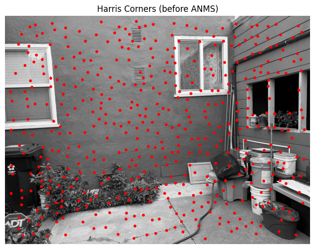
As specified in the paper Multi-Image Matching using Multi-Scale Oriented Patches, the Harris Corner Detector with Adaptive Non-Maximal Suppression can improve upon the manual process presented above. Below, we show a sample image without any detectors or filters applied, followed by an image where the Harris Corner Detector has been applied.
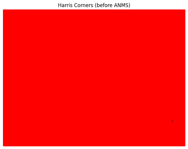
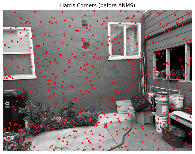
Uh oh! It seems there are too many interesting points — the algorithm has essentially captured almost every point visible in the image. Let’s increase min_distance to 100 to see if that improves the result:
We see more interesting results. In fact, if a human were to select points they consider important when matching corresponding pairs between this image and another taken from a different angle, they might choose a subset of the points shown here. However, we can do better — especially with the Adaptive Non-Maximal Suppression (ANMS) algorithm. Let’s take a look at the results:
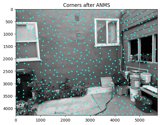
For comparison, if we randomly select 500 points from the image after applying the Harris Corner algorithm, we get the following:
We can clearly see that ANMS produces a much more spatially balanced and meaningful set of points.
Feature Descriptor Extraction
AMNS is still not good enough for our purpose. Although it helps extract interesting points, our ultimate goal is to identify interesting pairs of points that we can match. This allows us to perform automatic warping and create a visually appealing image.
Let’s move on and obtain some feature descriptors to assist with this process:
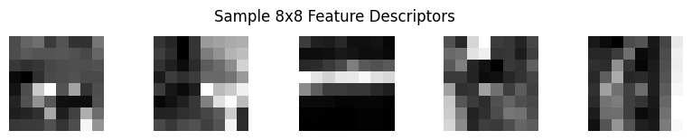
You can observe some interesting patterns here. The middle one appears to function somewhat like an edge detector, while the others seem to highlight regions where a particular pixel is brighter than most of the surrounding pixels in a given area.
Feature Matching
To narrow down our options and focus on matching only good features, we use Lowe’s thresholding with a value of 0.6. The following image shows the corresponding points connected by horizontal lines:
It’s a bit faint, but if you look closely, you can see the correspondences pretty clearly. See? I wasn’t lying when I said I took these pictures — they only differ by an angle!
Another example:
RANSAC for Robust Homography
Finally, to automatically generate clean-looking mosaic images (instead of manually selecting points — as shown in Part 1, which turned out quite messy), we use RANSAC for robust homography estimation. Below are the improved results:
For comparison, here’s the result using manually selected points (and, of course, since the points were a bit off):
The warping techniques differ slightly because I updated the code, but you can see that the middle area now has much less blurriness. This improvement comes from the automatic alignment being far more robust than my shaky manual selections.
Here are two more examples: