CS 180 Project 5: Fun With Diffusion Models!

Author

Wesley Zheng

Published

November 22, 2025

In this project, we will implement and deploy diffusion models for image generation.

Part A: The Power of Diffusion Models!

Part 0: Setup

For this project, we will be using the DeepFloyd IF Diffusion model. To start, we will explore some interesting prompts and their corresponding embeddings that may help us generate interesting images.

The following are some interesting prompts that I came up with (similar to those you might see in reels where people are playing around with diffusion models):

“a tranquil beach at dawn with soft pastel colors in the sky”
“a futuristic robot reading a newspaper in a cafe”
“a grand library with floating books and glowing runes”
“a snowy mountain village illuminated by lanterns at night”
“a deep-sea diver exploring a glowing coral cave”
“a dragon curled around a towering crystal spire”
“a vintage steam train crossing an old stone bridge”
“a tiny cottage surrounded by oversized magical mushrooms”
“a cybernetic wolf running through neon-lit streets”
“a peaceful meadow filled with fireflies at dusk”
“an explorer discovering ancient ruins in the desert”
“a spaceship docking at a colossal orbital station”
“a mystical forest with trees that emit bioluminescent light”
“a knight standing before a portal of swirling energy”
“a whimsical bakery run by anthropomorphic animals”

One can find the embeddings in the project notebook that I have created. For simplicity of the web page (knowing that embeddings are just a bunch of numbers), we will not show them here.

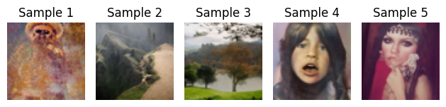
We will, however, show the initial results of the diffusion on the three prompts we chose:

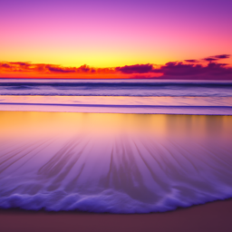
“a tranquil beach at dawn with soft pastel colors in the sky”

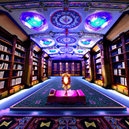
“a grand library with floating books and glowing runes”

“a futuristic robot reading a newspaper in a cafe”

In addition, we will also test different values of num_inferences. The images above used num_inferences = 20. The version below will use num_inferences = 1000, the maximum value we can achieve to see the image’s maximum potential, while we sacrifice time.

“a futuristic robot reading a newspaper in a cafe”

Interestingly enough, the three images that I generated initially all have a very “pink-shifted” appearance, but we never specified in the prompt that the image should have a pink shade. Perhaps this is because the initial randomized noise favored this color. In the num_inferences = 1000 version, the image is much different and probably fits the prompt much better (satisfying a normal person’s needs and expectations when they send the prompt). Overall, whether we use num_inferences = 20 or num_inferences = 1000, both reflect the prompt very well, as we can see that there is a robot, library, and beach.

The random seed that we will be using throughout the project is 180.

Part 1: Sampling Loops

1.1 Implementing the Forward Process

A key part is the forward function in the diffusion model. It can be summarized using the mathematical formula below:

\[ q(x_t | x_0) = N(x_t ; \sqrt{\bar\alpha} x_0, (1 - \bar\alpha_t)\mathbf{I}) \]

which is equivalent to computing:

\[ x_t = \sqrt{\bar\alpha_t} x_0 + \sqrt{1 - \bar\alpha_t} \epsilon \quad \text{where}~ \epsilon \sim N(0, 1) \]

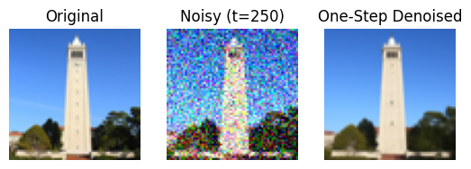
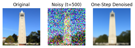
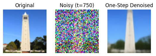
That is, given a clean image \(x_0\), we get a noisy image \(x_t\) at timestep \(t\) by sampling from a Gaussian with mean \(\sqrt{\bar\alpha_t} x_0\) and variance \((1 - \bar\alpha_t)\).

Below is the given campanile image (from UC Berkeley) at different noise levels:

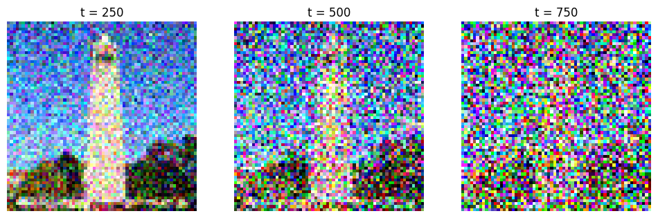
As we increase the noise level, the campanile is literally covered by the TV snowflakes that we will see, and it becomes harder to see the original image. But no worries! We will discover a way to take advantage of this in a moment.

1.2 Classical Denoising

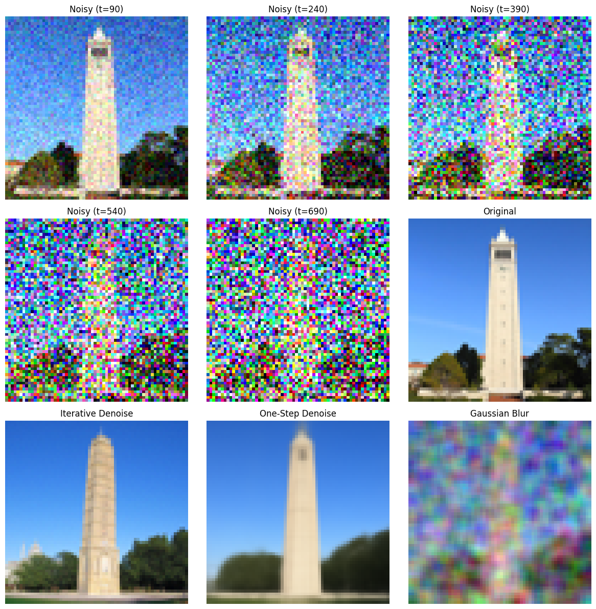
We will denoise the images using the classical Gaussian blur filtering we have seen in previous projects. For the sake of simplicity and saving space, we will not show the exact details. For some quick math, we are computing the high frequency and low frequency of the image separately and using that to deblur the image.

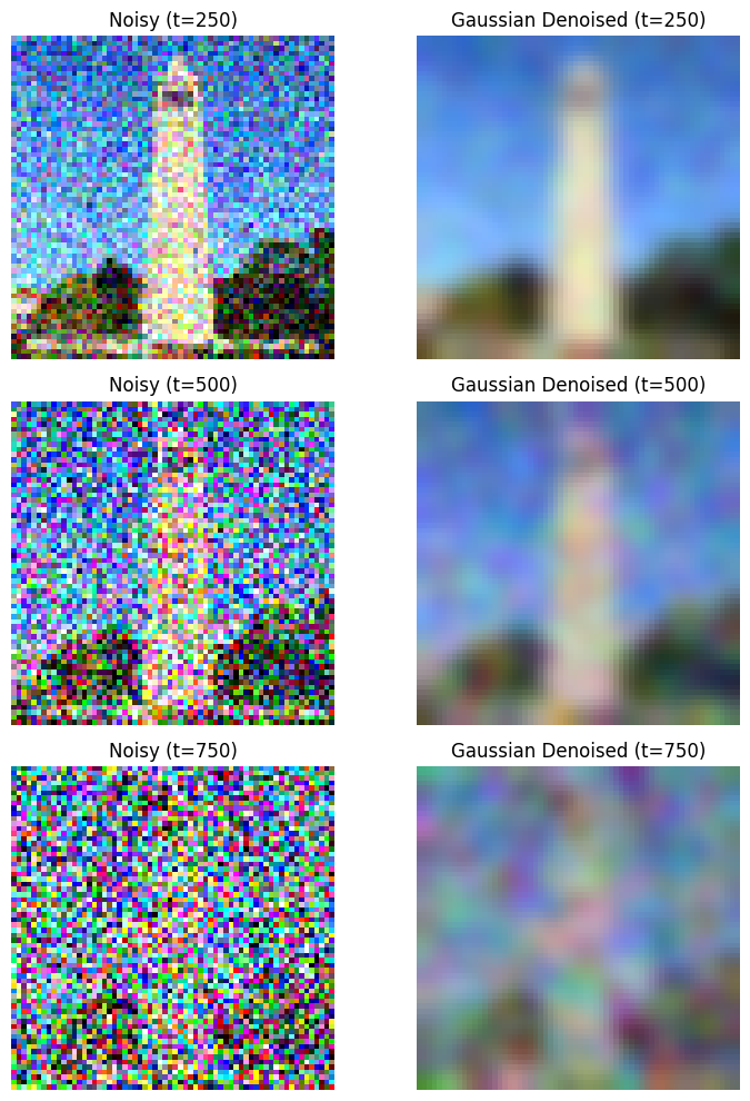
As we see above, it made the image somewhat better, though you can still see some noise in the picture.

1.3 One-Step Denoising

Gaussian deblurring is not doing enough, unfortunately. We will use more advanced techniques, such as using UNet, which can help us recover images from Gaussian noise. Let’s see the results.

1.4 Iterative Denoising

Building upon the previous subquestion, in theory, we could start with noise \(x_{1000}\) at timestep \(T = 1000\), denoise for one step to get an estimate of \(x_{999}\), and carry on until we get \(x_0\). However, we can skip steps to make it faster (in fact, my Colab cannot sustain so much since it will consume too many credits and money). We will be using the formula:

\[ x_{t'} = \frac{\sqrt{\bar\alpha_{t'}}\beta_t}{1 - \bar\alpha_t} x_0 + \frac{\sqrt{\alpha_t}(1 - \bar\alpha_{t'})}{1 - \bar\alpha_t} x_t + v_\sigma \]

where:

\(x_t\) is your image at timestep \(t\)
\(x_{t'}\) is your noisy image at timestep \(t'\) where \(t' < t\) (less noisy)
\(\bar\alpha_t\) is defined by alphas_cumprod
\(\alpha_t = \frac{\bar\alpha_t}{\bar\alpha_{t'}}\)
\(\beta_t = 1 - \alpha_t\)
\(x_0\) is our current estimate of the clean image using one-step denoising

\(v_\sigma\), as some might have guessed, represents the noise.

As a result, we get the following result:

1.5 Diffusion Model Sampling

Let’s generate some images from scratch and see how the diffusion models react. The only prompt we will give is “a high quality photo”.

Of course, we see that they are much different from the staff-referenced images. But this also means our methods are correct; it is very random—given just this prompt, the model could give anything.

1.6 Classifier-Free Guidance

CFG is a very good technique that will help us improve the image quality. In some sense, the image qualities generated from the pure diffusion model can be improved.

To start, CFG will edit the noise estimate, which can be found in the following equation:

\[ \epsilon = \epsilon_u + \gamma (\epsilon_c - \epsilon_u) \]

where \(\gamma\) controls the strength of CFG.

See the following images using the same “blank” prompt with the new technique that we have been hinted by the course staff:

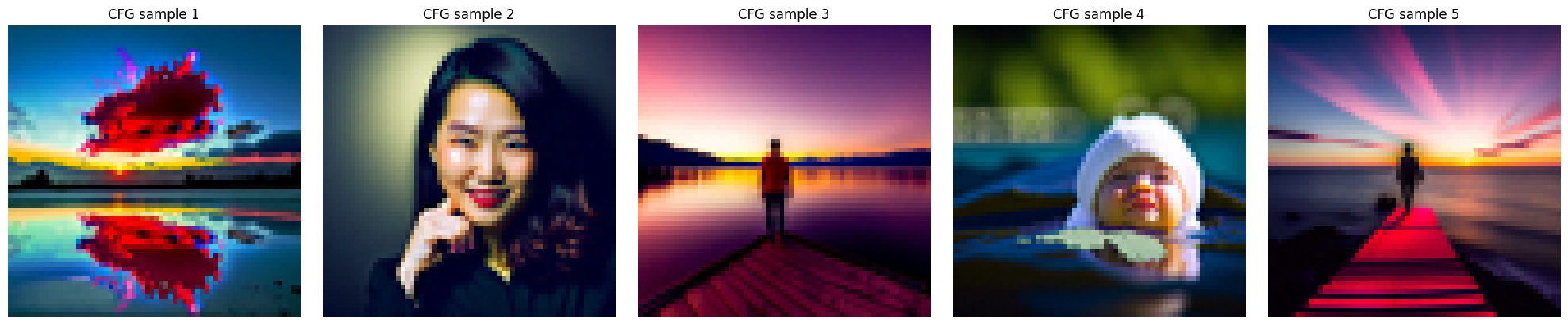
We see that the images are much more colorful and contain much more detail. Hopefully, that is a good sign that this technique will work, because we will be mainly using this technique in the following subproblems.

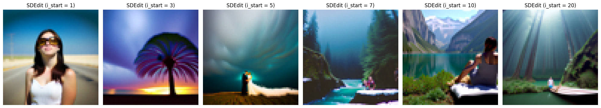
1.7 Image-to-image Translation

Now let’s try something more interesting. We want to replicate what is commonly seen in some reels: the gradual transition process from one image to another image, even if they seem very different at first. SD edit will be able to help us with this.

To start, we will be playing around with the campanile image, and start transitioning from a random image.

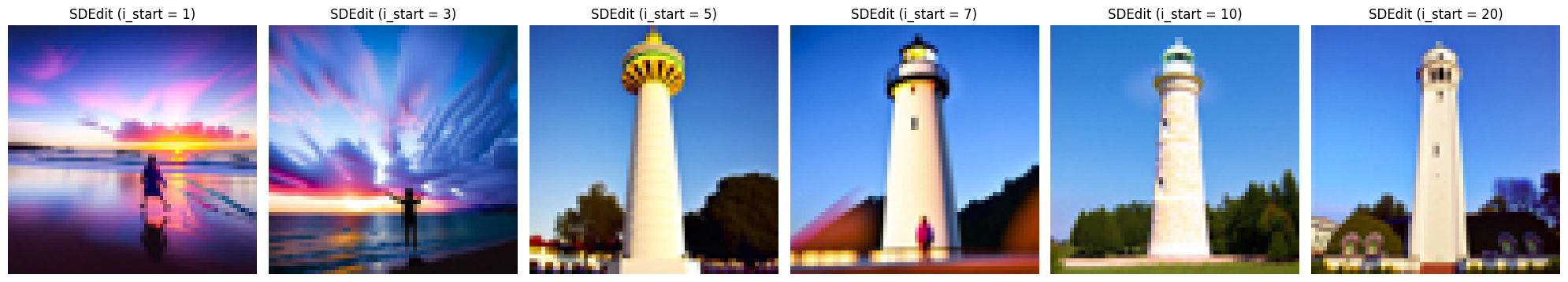
i_start = 3 to i_start = 5 seems a bit weird. I’m not sure why exactly the model had such a big difference there, as I, as a human being, could not see the visual similarity between these images that helped this transition, but here we go.

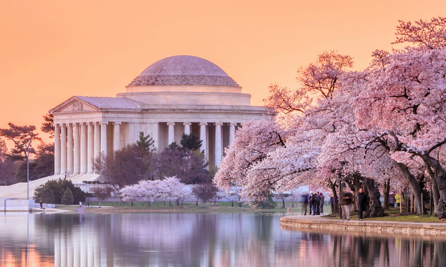
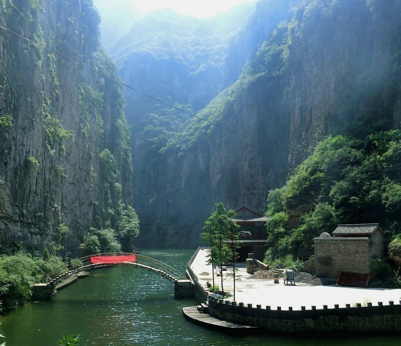
The following two image sequences are done on Washington, DC and Taiyuan images, places where I have lived for more than 5 years.

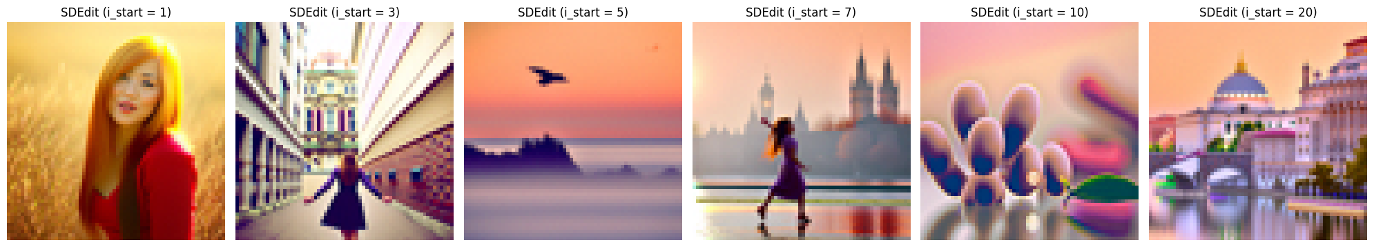
The Taiyuan one doesn’t make much sense, as it was supposed to show some building, but in the Washington, DC one you can somewhat see that it is the White House. Looks like our diffusion model is doing okay with this technique.

Here are the original pictures:

1.7.1 Editing Hand-Drawn and Web Images

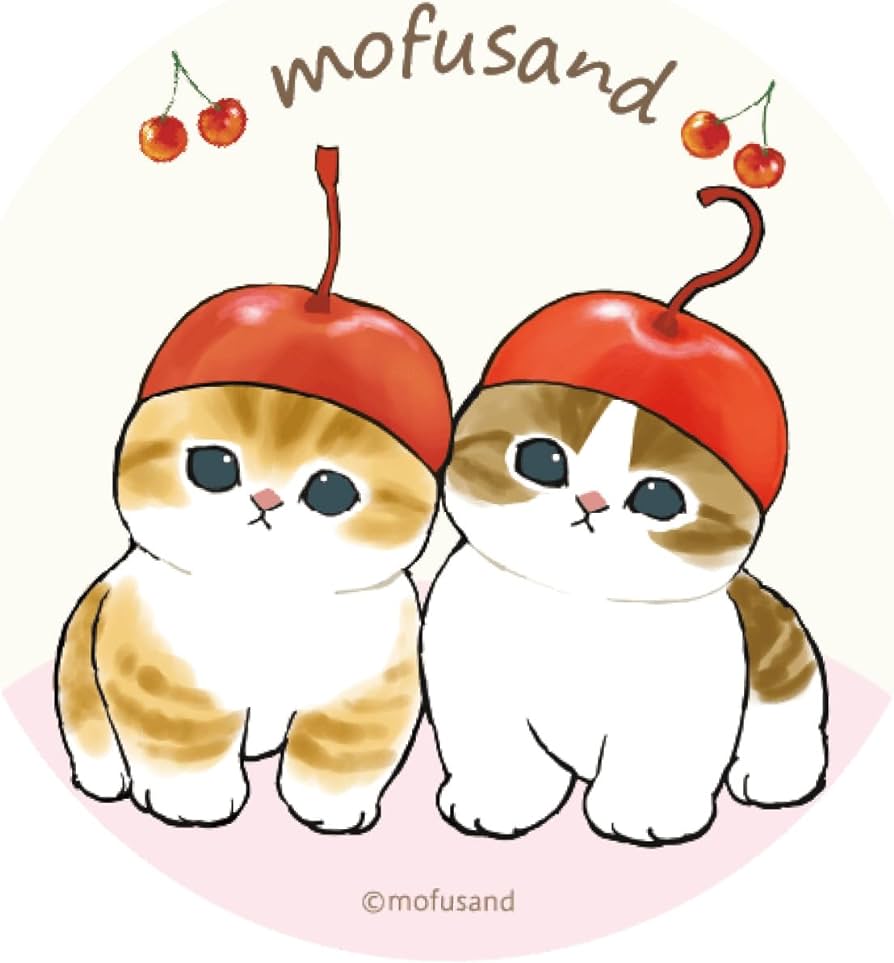
Let’s try playing with hand-drawn images and web images! Below, I will be using Mofusand art and two hand-drawn images (one boat on the sea and one butterfly—hopefully that’s pretty clear from the images).

The second-to-last image looks extremely close to the Mofusand image we provided. Though the final image looks somewhat off, looking from a far distance you probably cannot tell the difference. Below is the original picture:

Here are results on my hand-drawn images:

Here’s the original drawing:

Here’s the original drawing:

1.7.2 Inpainting

We will try inpainting, which is masking out some part of the image and asking the diffusion model to fill it up for us, which we probably will not get the original picture back. We will still be doing this on the campanile, Washington, and Taiyuan pictures.

For Taiyuan, we will be masking out the existence of the boat, and see what the model can generate:

Very blurry but it seems like it has been changed to forest.

We will mask out the White House:

Very random. It seems like it has been replaced with cherry blossoms, which I guess isn’t so bad.

1.7.3 Text-Conditional Image-to-image Translation

Instead of prompting from a blank/random image, we will start off from an image with our own prompt.

From “a snowy mountain village illuminated by lanterns at night” to the Campanile:

From “a snowy mountain village illuminated by lanterns at night” to Washington:

From “a snowy mountain village illuminated by lanterns at night” to Taiyuan:

1.8 Visual Anagrams

We will be generating some anagrams! Though I didn’t get them to be as decent as the staff solutions, here are some interesting ones:

a tranquil beach at dawn with soft pastel colors in the sky

a futuristic robot reading a newspaper in a cafe

a tiny cottage surrounded by oversized magical mushrooms

a snowy mountain village illuminated by lanterns at night

1.9 Hybrid Images

We have done hybrid images in previous projects. We will be replicating that with CFG. To be specific, the algorithm will be:

\[ \begin{align} \epsilon_1 &= \text{CFG of UNet}(x_t, t, p_1) \\ \epsilon_2 &= \text{CFG of UNet}(x_t, t, p_2) \\ \epsilon &= f_\text{lowpass}(\epsilon_1) + f_\text{highpass}(\epsilon_2) \end{align} \]

where UNet is the diffusion model UNet, \(f_\text{lowpass}\) is a low-pass function, \(f_\text{highpass}\) is a high-pass function, and \(p_1\) and \(p_2\) are two different text prompt embeddings. Our final noise estimate is \(\epsilon\).

To end Part A, here are our sample hybrid images:

a deep-sea diver exploring a glowing coral cave + a knight standing before a portal of swirling energy

a tranquil beach at dawn with soft pastel colors in the sky + a snowy mountain village illuminated by lanterns at night

Part B: Flow Matching from Scratch!

In this part, we will build and train a UNet using the MNIST dataset. The workflow feels very similar to what you might have seen in classes such as CS 189, so it serves as a nice cool down after Part A.

Part 1: Training a Single-Step Denoising UNet

We start by creating a simple one-step denoiser. Our goal is to map a noisy image back to a clean image so the digit is recognizable again. The denoiser is trained with the following mean squared error loss:

\[ L = \mathbb{E}_{z,x} \|D_{\theta}(z) - x\|^2 \]

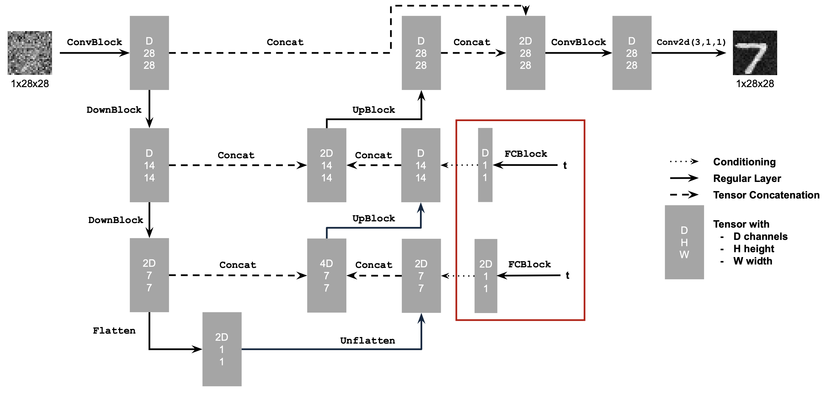
1.1 Implementing the UNet

The architecture of the UNet we construct is shown below:

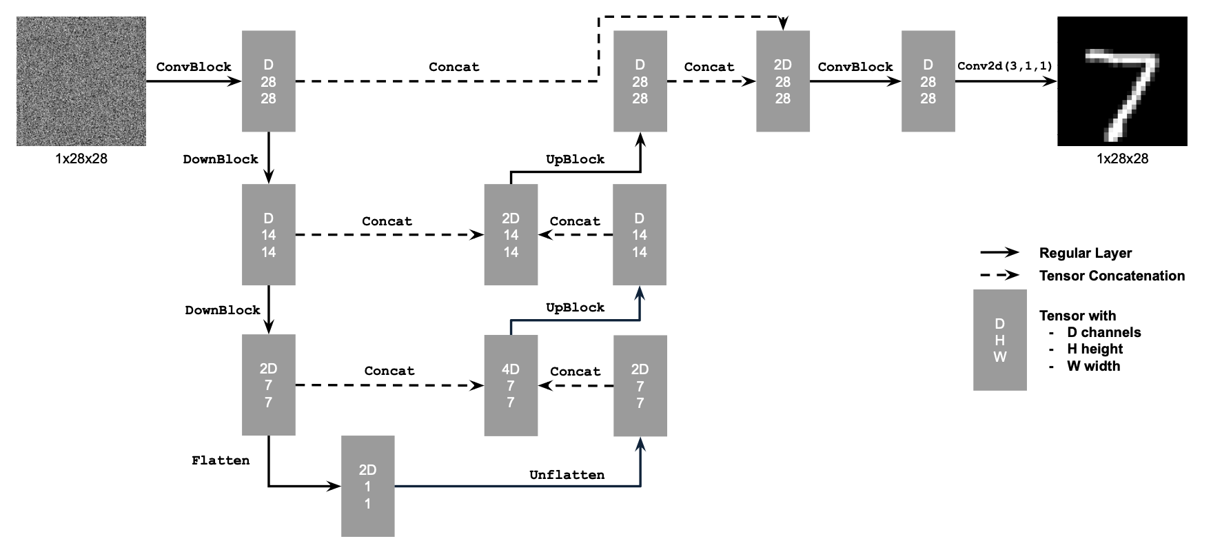
Visually, it becomes clear which layers and channel dimensions we need.

The following diagram explains what each operation does:

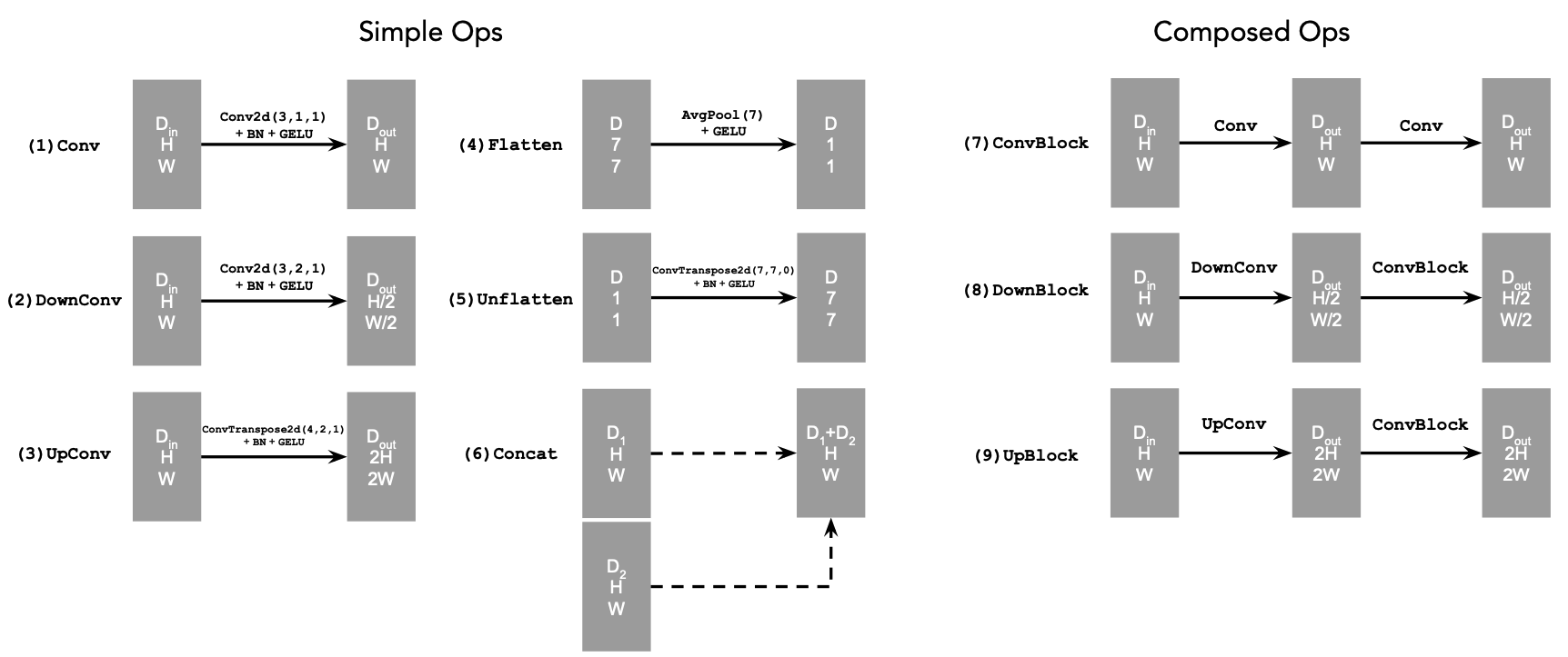
In summary,

Conv keeps the spatial resolution constant while changing the channel dimension.
DownConv downsamples the tensor by a factor of 2.
UpConv upsamples the tensor by a factor of 2.
Flatten averages a 7×7 tensor into a 1×1 tensor (7 is the size after the downsampling stages).
Unflatten upsamples a 1×1 tensor back to 7×7.
Concat performs a channel-wise concatenation of tensors with the same height and width via torch.cat().

1.2 Using the UNet to Train a Denoiser

Now that the architecture is settled, we can generate noisy/clean training pairs with:

\[ z = x + \sigma \epsilon,\quad \text{where }\epsilon \sim N(0, I) \]

Here, \(z\) is the noisy image and \(x\) is the original clean digit. Varying \(\sigma\) lets us visualize how the noise level affects image quality:

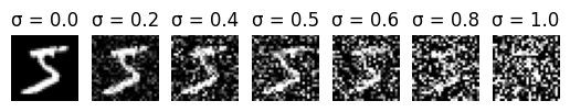
As expected, increasing the noise level gradually destroys the semantic content—the digit becomes harder and harder to recognize.

1.2.1 Training

With this synthetic dataset in place, we train the UNet denoiser and monitor how quickly it reconstructs digits across different noise scales. Let’s see the results:

Denoised Results after 1 epoch

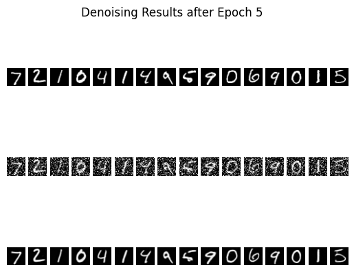Denoised Results after 5 epochs

Even after just one epoch the reconstructions already resemble the ground-truth digits, and by epoch five the digits are mostly clean with only mild residual noise. That level of fidelity is good enough for our purposes because a human—or any downstream classifier—can reliably read the digit classes from these predictions.

Let’s also look at the training curve to get a general sense of how the model improves over epochs and iterations:

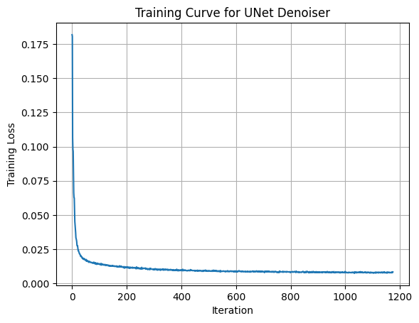
The model is not overfitting: the qualitative samples shown above come from the validation set, and the validation loss closely tracks the training curve.

1.2.2 Out-of-Distribution Testing

Note that the UNet was trained with \(\sigma = 0.5\). To check whether it overfits to that particular corruption level, I ran the same checkpoint on alternative values without retraining:

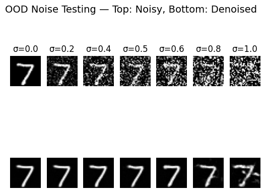
Lower noise levels (\(\sigma = 0.2\)) are reconstructed almost perfectly, while higher ones (\(\sigma = 0.8\)) look blurrier yet still capture the correct digit structure. Other than the extreme \(\sigma = 1.0\) case, the model behaves consistently well across the tested noise scales, which is encouraging.

1.2.3 Denoising Pure Noise

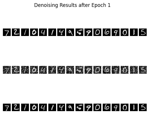
Next, I removed the fixed-\(\sigma\) assumption altogether. Instead of sampling a single noise magnitude, each training example now receives Gaussian noise drawn directly from \(\mathcal{N}(0, I)\). This setting is much harder because the network must learn to denoise across a continuum of corruption levels.

Epoch 1 Results

Epoch 5 Results

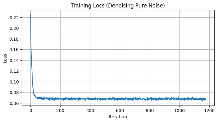
The corresponding loss curve is shown below:

Interestingly, the qualitative results lag behind the fixed-\(\sigma\) experiment even though the loss decreases steadily. Zooming in does reveal minor improvements between epoch 1 and epoch 5, but the gains are modest. This makes sense: removing the stable \(\sigma = 0.5\) setting forces the model to generalize across highly variable noise magnitudes, which is simply a tougher problem. The good news is that this limitation does not block the later experiments—we can still reuse the insights from this section going forward.

Part 2: Training a Flow Matching Model

Now we move into the flow-matching setting so we can iteratively denoise images rather than relying on a single-step model. The core interpolation formula we will use is:

\[ x_t = (1-t)x_0 + tx_1 \quad \text{where } x_0 \sim \mathcal{N}(0, 1), t \in [0, 1] \]

Flow describes the velocity of the vector field produced by this interpolation. In other words,

\[ u(x_t, t) = \frac{d}{dt} x_t = x_1 - x_0 \]

Our training objective becomes:

\[ \begin{equation} L = \mathbb{E}_{x_0 \sim p_0(x_0), x_1 \sim p_1(x_1), t \sim U[0, 1]} \|(x_1-x_0) - u_\theta(x_t, t)\|^2 \end{equation} \]

2.1 Adding Time Conditioning to UNet

To make the UNet time-aware, we follow the course-staff diagram below. The extra inputs allow the network to receive both the noised sample \(x_t\) and the timestep \(t\) so it can predict the flow vector conditioned on time.

We also introduce the fully connected (FC) block that embeds the time signal before injecting it into the convolutional stack:

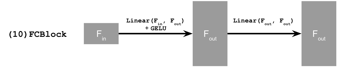
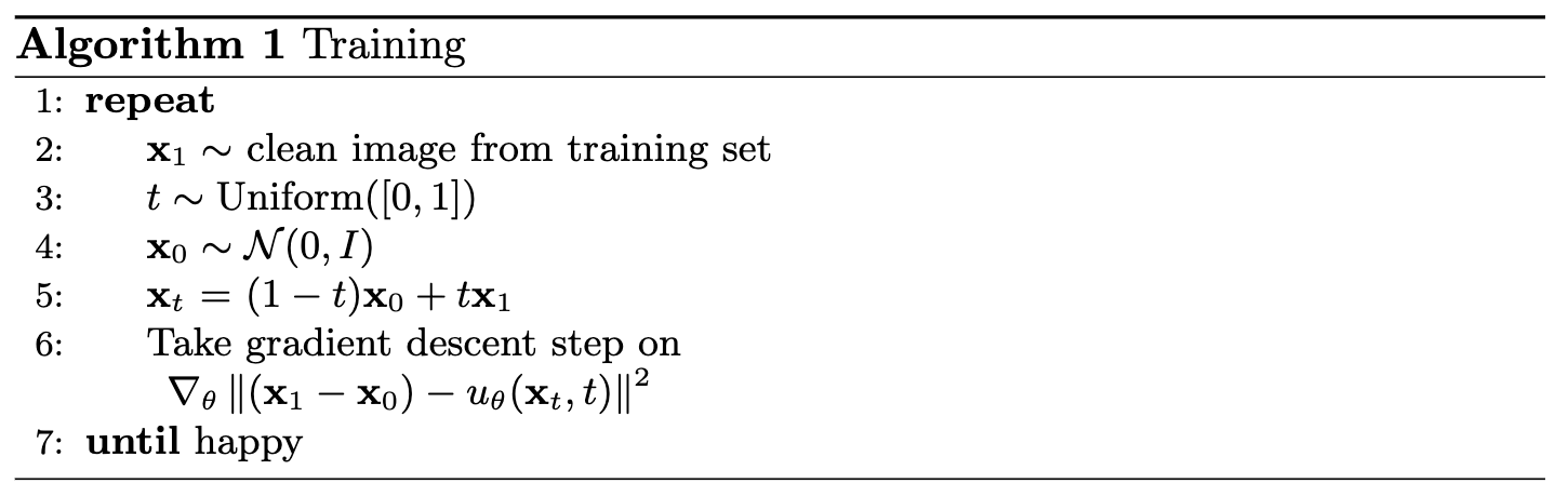
2.2 Training the UNet

With the architecture in place, we train according to the algorithm below (essentially Algorithm 1 from the project handout):

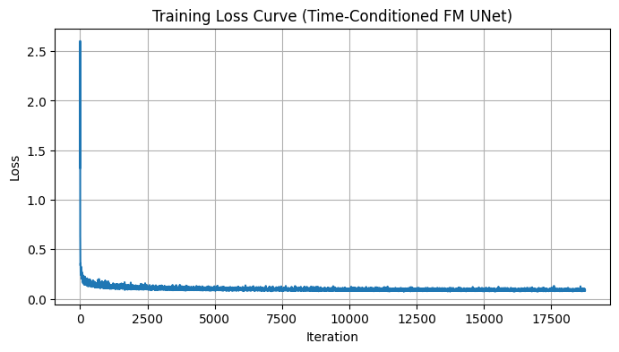
The model’s performance over a few epochs is summarized in the loss curve:

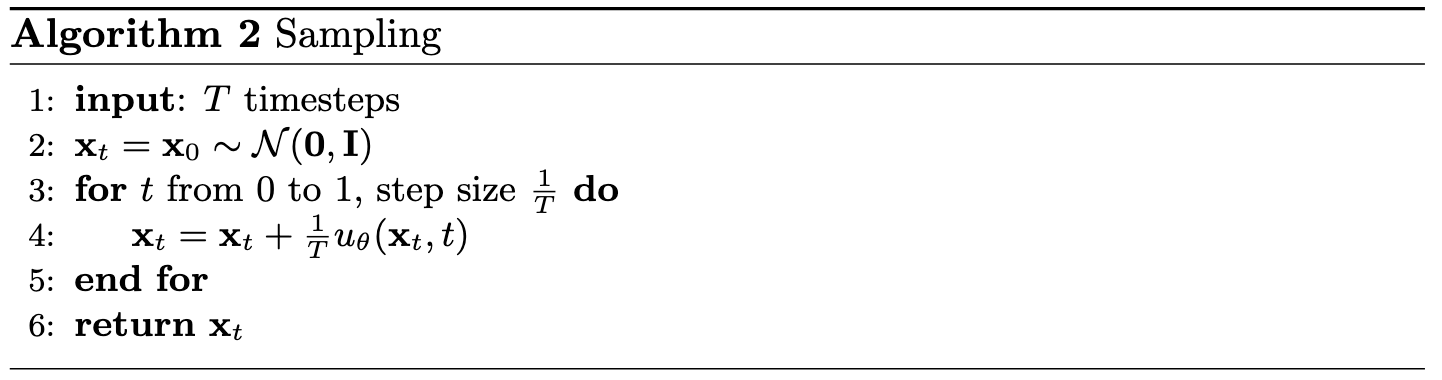
2.3 Sampling from the UNet

With the flow-trained UNet in hand, we can now run iterative denoising to sample new digits. The procedure (Algorithm 2 in the handout) repeatedly predicts the flow vector and takes a small Euler step toward the data distribution:

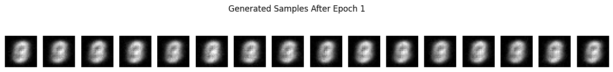
Results after 1, 5, and 10 epochs of training are shown below. The samples sharpen noticeably as training progresses, though there is still room for improvement in global coherence:

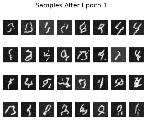Epoch 1 Results

Epoch 5 Results

Epoch 10 Results

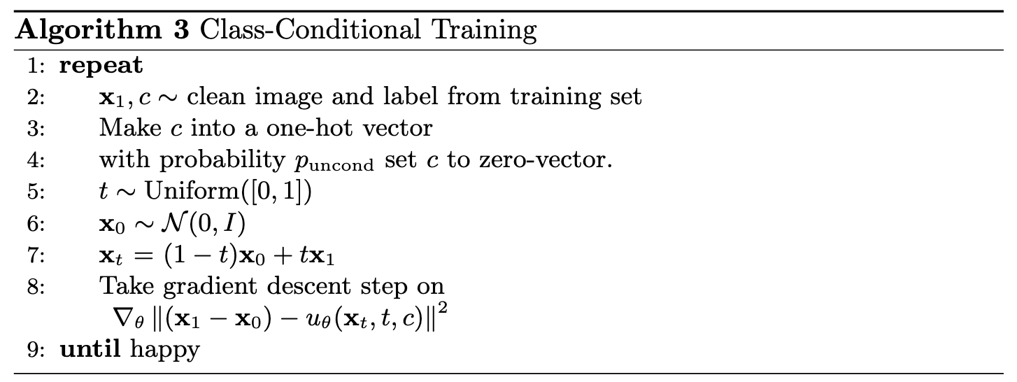
2.4 Adding Class-Conditioning to UNet

To push sample quality further, we feed the digit label into the network so it can specialize its predictions per class. This is analogous to CFG in diffusion models: conditioning provides a stronger signal that helps the model stay on-manifold.

2.5 Training the UNet

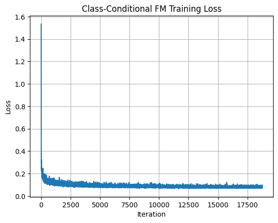
With class-conditioning enabled, we train using the procedure shown below:

The updated training loss exhibits more variance toward the end, likely because the conditional model has greater capacity:

2.6 Sampling from the UNet

Using the conditional sampler (Algorithm 4), we can now generate digits for specific classes:

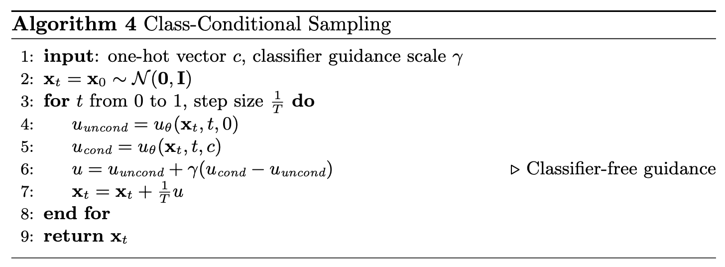
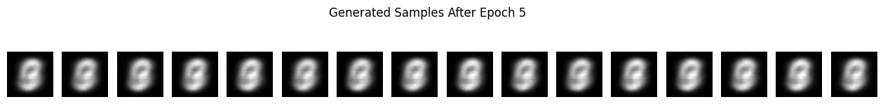
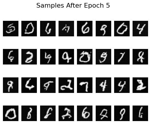
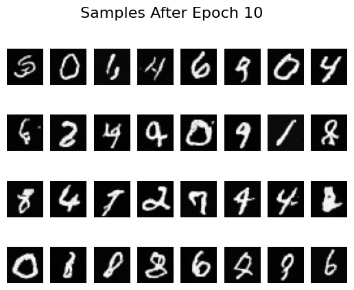
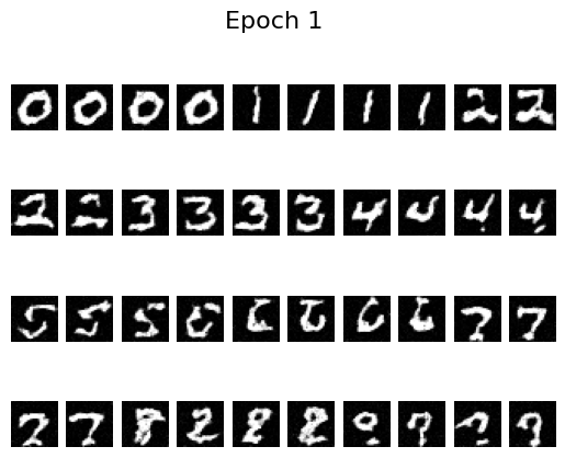
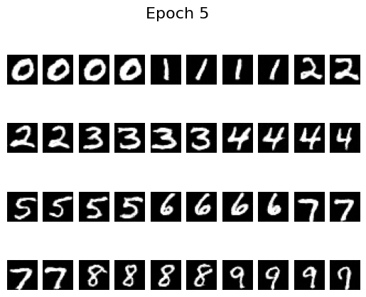
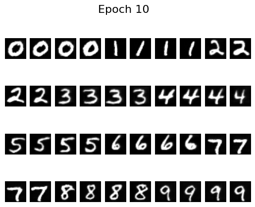
Samples after different numbers of epochs illustrate how quickly the model improves:

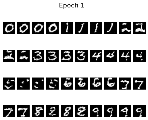Epoch 1 Epoch 1

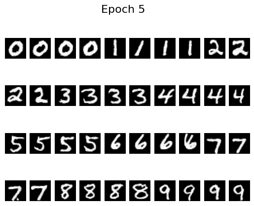Epoch 5 Epoch 5

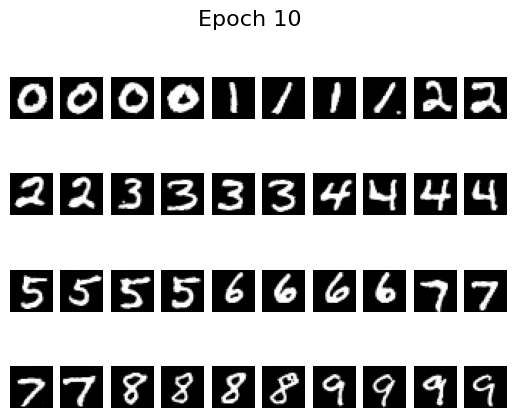Epoch 10

By epoch 5 the digits are already crisp, helped by the scheduler that decays the learning rate. To see whether we can remove that scheduler, I retrained with a fixed learning rate of \(10^{-4}\) (instead of \(10^{-2}\)) and added gradient clipping via torch.nn.utils.clip_grad_norm_(fm.parameters(), 1.0). The results remain stable without the scheduler:

Epoch 1 Epoch 1

Epoch 5 Epoch 5

Epoch 10

And that wraps up the final project of the semester!