49 Discussion 09: Particle Filtering and Naive Bayes (From Spring 2025)
49.1 Particle Filtering
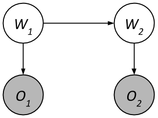
Let’s use Particle Filtering to estimate the distribution of \(P(W_2 \mid O_1 = a, O_2 = b)\). Here’s the HMM again. \(O_1\) and \(O_2\) are supposed to be shaded.
| \(W_1\) | \(P(W_1)\) |
|---|---|
| 0 | 0.3 |
| 1 | 0.7 |
| \(W_t\) | \(W_{t+1}\) | \(P(W_{t+1}\mid W_t)\) |
|---|---|---|
| 0 | 0 | 0.4 |
| 0 | 1 | 0.6 |
| 1 | 0 | 0.8 |
| 1 | 1 | 0.2 |
| \(W_t\) | \(O_t\) | \(P(O_t \mid W_t)\) |
|---|---|---|
| 0 | a | 0.9 |
| 0 | b | 0.1 |
| 1 | a | 0.5 |
| 1 | b | 0.5 |
We start with two particles representing our distribution for \(W_1\):
- \(P_1: W_1 = 0\)
- \(P_2: W_1 = 1\)
Use the following random numbers to run particle filtering:
49.1.1 (a)
Observe: Compute the weight of the two particles after evidence \(O_1 = a\)
Answer
\[ w(P_1) = P(O_1 = a \mid W_1 = 0) = 0.9 \]
\[ w(P_2) = P(O_1 = a \mid W_1 = 1) = 0.5 \]49.1.2 (b)
Resample: Using the random numbers, resample \(P_1\) and \(P_2\) based on the weights
Answer
We sample from the weighted distribution above. Using the first two random samples:
\[ P_1 = sample(\text{weights}, 0.22) = 0 \]
\[ P_2 = sample(\text{weights}, 0.05) = 0 \]49.1.3 (c)
Predict: Sample \(P_1\) and \(P_2\) from applying the time update
Answer
\[ P_1 = sample(P(W_{t+1} \mid W_t = 0), 0.33) = 0 \]
\[ P_2 = sample(P(W_{t+1} \mid W_t = 0), 0.20) = 0 \]49.1.4 (d)
Update: Compute the weight of the two particles after evidence \(O_2 = b\)
Answer
\[ w(P_1) = P(O_2 = b \mid W_2 = 0) = 0.1 \]
\[ w(P_2) = P(O_2 = b \mid W_2 = 0) = 0.1 \]49.1.5 (e)
Resample: Using the random numbers, resample \(P_1\) and \(P_2\) based on the weights
Answer
Because both particles have \(W_2 = 0\), resampling leaves both particles unchanged:
\[ P_1 = 0 \]
\[ P_2 = 0 \]49.1.6 (f)
What is our estimated distribution for \(P(W_2 \mid O_1 = a, O_2 = b)\)
Answer
\[ P(W_2 = 0 \mid O_1 = a, O_2 = b) = \frac{2}{2} = 1 \]
\[ P(W_2 = 1 \mid O_1 = a, O_2 = b) = \frac{0}{2} = 0 \]49.2 Naive Bayes
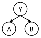
In this question, we will train a Naive Bayes classifier to predict class labels \(Y\) as a function of input features \(A\) and \(B\). \(Y\), \(A\), and \(B\) are all binary variables, with domains 0 and 1. We are given 10 training points from which we will estimate our distribution.
| \(A\) | 1 | 1 | 1 | 1 | 0 | 1 | 0 | 1 | 1 | 1 |
|---|---|---|---|---|---|---|---|---|---|---|
| \(B\) | 1 | 0 | 0 | 1 | 1 | 1 | 1 | 0 | 1 | 1 |
| \(Y\) | 1 | 1 | 0 | 0 | 0 | 1 | 1 | 0 | 0 | 0 |
49.2.1 (a)
What are the maximum likelihood estimates for the tables \(P(Y)\), \(P(A|Y)\), and \(P(B|Y)\)?
| \(Y\) | \(P(Y)\) |
|---|---|
| 0 | |
| 1 |
| \(A\) | \(Y\) | \(P(A|Y)\) |
|---|---|---|
| 0 | 0 | |
| 1 | 0 | |
| 0 | 1 | |
| 1 | 1 |
| \(B\) | \(Y\) | \(P(B|Y)\) |
|---|---|---|
| 0 | 0 | |
| 1 | 0 | |
| 0 | 1 | |
| 1 | 1 |
Answer
| \(Y\) | \(P(Y)\) |
|---|---|
| 0 | 3/5 |
| 1 | 2/5 |
| \(A\) | \(Y\) | \(P(A|Y)\) |
|---|---|---|
| 0 | 0 | 1/6 |
| 1 | 0 | 5/6 |
| 0 | 1 | 1/4 |
| 1 | 1 | 3/4 |
| \(B\) | \(Y\) | \(P(B|Y)\) |
|---|---|---|
| 0 | 0 | 1/3 |
| 1 | 0 | 2/3 |
| 0 | 1 | 1/4 |
| 1 | 1 | 3/4 |
49.2.2 (b)
Consider a new data point (\(A = 1\), \(B = 1\)). What label would this classifier assign to this sample?
Answer
\[ P(Y=0, A=1, B=1) = P(Y=0)P(A=1|Y=0)P(B=1|Y=0) = (3/5)(5/6)(2/3) = 1/3 \]
\[ P(Y=1, A=1, B=1) = P(Y=1)P(A=1|Y=1)P(B=1|Y=1) = (2/5)(3/4)(3/4) = 9/40 \]
Our classifier will predict label 0.49.2.3 (c)
Let’s use Laplace Smoothing to smooth out our distribution. Compute the new distribution for \(P(A|Y)\) given Laplace Smoothing with \(k=2\).
| \(A\) | \(Y\) | \(P(A|Y)\) |
|---|---|---|
| 0 | 0 | |
| 1 | 0 | |
| 0 | 1 | |
| 1 | 1 |
Answer
| \(A\) | \(Y\) | \(P(A|Y)\) |
|---|---|---|
| 0 | 0 | 3/10 |
| 1 | 0 | 7/10 |
| 0 | 1 | 3/8 |
| 1 | 1 | 5/8 |