Code
import numpy as np
from datascience import *
%matplotlib inline

amounts = np.random.normal(loc=2.5, scale=1, size=150)
amounts = np.clip(amounts, 0.5, 7)

water = Table().with_columns(
    "amount", amounts
)| Name | Wesley Zheng |
| Pronouns | He/him/his |
| wzheng0302@berkeley.edu | |
| Discussion | Wednesdays, 12–2 PM @ Etcheverry 3105 |
| Office Hours | Tuesdays/Thursdays, 2–3 PM @ Warren Hall 101 |
Contact me by email at ease — I typically respond within a day or so!
Congrats on finishing the midterm!
What has been your favorite topic, assignment, lecture, or anything so far with the first half of the class done? Please leave any comments you have about the content and any feedback for your TA here. Tear this page off and fold it so it is anonymous.
Additionally, if you have any concerns about your performance in the class so far, feel free to bring it up with your TA in person, or via email.
Setup
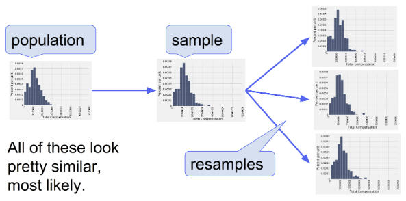
We want to be able to produce an estimate of a particular population parameter of interest, say the median. However, we know that if we had gotten a different sample, then our estimate of the population median could have also been different.
Main Objective
If we were satisfied with our sample, we could simply take the statistic of the sample and call it the prediction for the population median. Even though this is a valid approximation method, we want to use the method of the bootstrap to generate a range of values for which we believe our population parameter falls into.
Method
Ideally, we would be able to take more samples from the population and find estimates for the population parameter in all of these samples. However, we are usually not able to resample from the original population due to resource constraints, necessitating the process of the bootstrap.
When we conduct a bootstrap resample, what size resample should we draw from our sample? Why?
Why do we need to resample from our sample with replacement?
When we conduct a bootstrap resample, what is the underlying assumption/reasoning for resampling from our sample? Why does it work?
Warm Up: What is the difference between a parameter and a statistic? Which of the two is random?
You are interested in investigating the liters of water consumed every day by UC Berkeley students. In particular, you want to study the proportion of students drinking less than 3 liters of water per day. You contact 150 random students from the directory and obtain the amounts of water each one of them drinks, storing them in the table water. The table has 1 column, amount, which stores the number of liters of water drunk by each student.
import numpy as np
from datascience import *
%matplotlib inline
amounts = np.random.normal(loc=2.5, scale=1, size=150)
amounts = np.clip(amounts, 0.5, 7)
water = Table().with_columns(
"amount", amounts
)What is the parameter and what is the statistic in this scenario?
Parameter: The proportion of UC Berkeley students who drink less than 3 liters of water per day.
Statistic: The proportion of students in the sample who drink less than 3 liters of water per day.Write a line of code to calculate the proportion of students in your sample who drank less than 3 liters of water per day.
np.mean(water.column("amount") < 3)0.70666666666666667Write a line of code to perform a single bootstrap resample of the data stored in the water table.
water.sample(water.num_rows, with_replacement = True)| amount |
|---|
| 2.58785 |
| 2.57834 |
| 4.79749 |
| 2.50783 |
| 1.89741 |
| 0.976994 |
| 3.05076 |
| 1.63481 |
| 2.48673 |
| 1.63481 |
... (140 rows omitted)
Alternatively, given the default values of the arguments, you may simply write
water.sample()| amount |
|---|
| 3.53367 |
| 3.42822 |
| 4.23784 |
| 3.40573 |
| 2.71503 |
| 2.05936 |
| 1.78597 |
| 5.01298 |
| 2.72281 |
| 4.79749 |
... (140 rows omitted)
Fill in the following blanks to conduct 10,000 bootstrap resamples of your data, calculating the proportion of students in each resample that drink less than 3 liters of water per day, then plotting the distribution of those proportions using an appropriate visualization.
proportions = _______________
for i in _______________:
  resampled_table = ________________________________
  resampled_statistic = __________________________
  proportions = _____________________________
proportions_table = Table().with_column("Resampled proportions", proportions)
proportions_table._______________proportions = make_array()
for i in np.arange(10000):
resampled_table = water.sample(water.num_rows, with_replacement=True)
resampled_statistic = np.mean(resampled_table.column("amount") < 3)
proportions = np.append(proportions, resampled_statistic)
proportions_table = Table().with_column("Resampled proportions", proportions)
proportions_table.hist("Resampled proportions")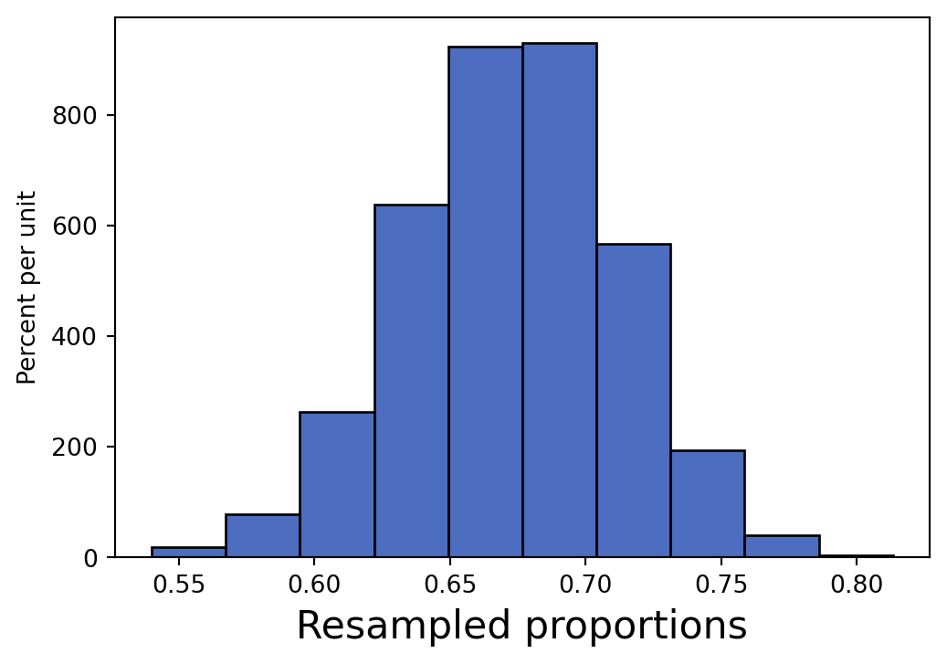
Ciana is interested in exploring the heights of women’s tennis players. She has collected a sample of 100 heights of professional women’s tennis players and wants to use this sample to estimate the true interquartile range (IQR) of all heights of professional women’s tennis players.
We define the interquartile range (IQR) as:
heights = np.random.normal(loc=175, scale=7, size=100)

tennis = Table().with_columns(
    "Height (cm)", heights
)In order to construct a 99% confidence interval for the IQR, what should our upper and lower endpoints be in terms of percentiles?
Our lower endpoint should be the 0.5th percentile and the upper endpoint should be the 99.5th percentile.
Define a function ci_iqr that constructs a 99% confidence interval for the IQR and returns an array containing the left endpoint and right endpoint of the 99% confidence interval in that order. The function takes in the following arguments:
tbl: A one-column table consisting of a random sample from the population; you can assume this sample is large.reps: The number of bootstrap repetitions.To find the 25th and 75th percentile of an array, you can use the percentile function.
Fill in the blanks and then provide the full solution.
def ci_iqr(tbl, reps):
stats = _______________
  for ________________:
    resample_col = ________________________________
    new_iqr = _________________________________
    stats = __________________________________
  left_end = _______________
  right_end = ______________
return ______________def ci_iqr(tbl, reps):
stats = make_array()
for i in np.arange(reps):
resample_col = tbl.sample().column(0)
new_iqr = percentile(75, resample_col) - percentile(25, resample_col)
stats = np.append(stats, new_iqr)
left_end = percentile(0.5, stats)
right_end = percentile(99.5, stats)
return make_array(left_end, right_end)ci_iqr(tennis, 100)array([ 5.7866864 , 11.90003896])Say Ciana recruited 500 of her friends to perform the same bootstrapping process she did. In other words, each of her friends drew a large, random sample of 100 heights from the population of professional women’s tennis players and constructed their own 99% confidence intervals.
Approximately how many of these CIs do we expect to contain the actual IQR for the heights of professional women’s tennis athletes?
We interpret a 99% confidence interval to mean that we are 99% confident in the process used to construct that given interval. In other words, 99% of the time we use this process we expect to construct an interval that contains the true population parameter.
Since we have 500 CIs, each at a 99% confidence level, we find that since \(500 \cdot (0.99) = 495\), we expect to have 495 of these CIs containing the actual IQR of heights.Note how in this example, we obtain different random samples from the population for each confidence interval, and then re-sample from each to produce a confidence interval.
Why each person not just re-use the same original sample? Why is this distinction important?
Ciara decided to do this process again, but this time with only 50 of her friends. Would the number of CIs that contain the actual IQR be more or less close to the expected number of CIs, compared to her results with 500 friends?
Ciara now decides to perform a hypothesis test, with the null hypothesis that the true IQR is q.
How could Ciara perform this using her confidence intervals? Discuss the duality of confidence intervals and hypothesis testing.
The confidence interval describes the region for which we can be 99% confident that it contains the true population parameter. This describes exactly the error of the p-value cutoff.
The decision rule for a hypothesis test testing whether the IQR is q could therefore be
If Ciara conducted a two-tailed hypothesis test (e.g. her alternative was “the IQR is not q”), what p-value cutoff would she choose if she used her confidence intervals?
If Ciara conducted a one-tailed hypothesis test (e.g. her alternative was “the IQR is greater than q”), what p-value cutoff would she choose if she used her confidence intervals?
The effective cutoff should be 0.5%, since we construct 99% confidence intervals, but only look at one tail. This is true since the confidence intervals we generate will have equal tails*, and therefore the same probability, so we can halve the tail region.
Typically, we would choose a p-value cutoff first, such as of 1% and then construct 98% confidence intervals to determine the outcome of the test. For the purposes of this question, we used the same confidence interval for both part (v) and part (vi).
*Note: bootstrapped percentile confidence intervals have equal tails, but may not be symmetric. Confidence intervals generated in other ways, not taught in Data 8, may not have equal tails.