Create a table containing Type and Generation that is sorted in decreasing order by the average HP for each pair of Type and Generation that appears in the table.
Return an array that contains ratios of legendary to non-legendary pokemons for each generation. You may assume that the Legendary column is a column of booleans.
Consider another table called trainers, which contains information about Pokemon trainers and the Pokemon they own. The trainers table has two columns: Trainer, the name of the trainer and Pokemon, the name of the Pokemon. Use table operations to create a new table called pokemon_with_trainers that includes each Pokemon’s Name, Type, Generation, and their Trainer.
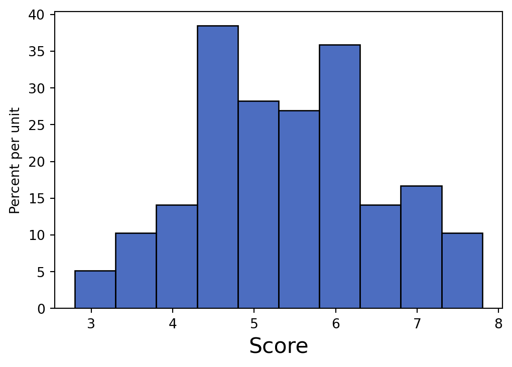
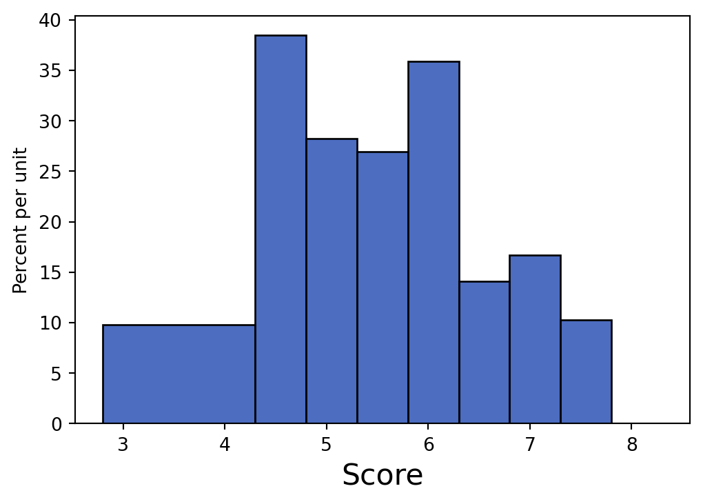
World Happiness Report is a landmark study on the state of global happiness. This study calculated and ranked the happiness level for 155 countries using data from the Gallup World Poll. The histogram below shows the distribution of happiness scores computed from this study in 2019. Suppose the data is stored in the table called happiness. The following code was used to generate the histogram you see below:
Note that the histogram may look a bit different from usual for the purpose of making bar heights easier to interpret.
NoteThinking About Histograms
Remember the area principle: the area of each bar corresponds to its proportion of the data.
We don’t know how values are distributed within a single bin — only the count (or percent) of values in that bin.
Without the actual counts, a histogram only gives us percentages, not raw numbers.
20.2.1 (a)
What are the units of the y-axis in the histogram?
Answer
Percent per happiness score. Note that it is NOT “percent per country”. Although each data point used to generate the histogram represents a country, the values used to make the histogram are the happiness scores.
For part b - e, use the above histogram to calculate the following quantities. If it’s not possible, write “Cannot calculate” and explain your reasoning.
20.2.2 (b)
The proportion of countries with happiness scores between 4.3 and 5.8.
Answer
Each bin has width 0.5. We’re interested in the [4.3, 4.8), [4.8, 5.3), and [5.3, 5.8)] bins, which have heights approximately 38, 28, and 27 percent per unit respectively. We can use the Area Principle to calculate the sum of the areas of these bins, which in turn represents the proportion we’re looking for: \[
\begin{align*}
\text{Total Area} &= \text{height}_1 \cdot \text{width} + \text{height}_2 \cdot \text{width} + \text{height}_3 \cdot \text{width} \\
&= 0.5 \cdot (\text{height}_1 + \text{height}_2 + \text{height}_3) \\
&= 0.5 \cdot (38 + 28 + 27) \\
&= 0.5 \cdot 93 \\
&= 46.5\% \quad \text{or as a proportion, } 0.465
\end{align*}
\]
The number of countries with happiness scores between 4.3 and 5.8 (round to the nearest country).
Answer
We can simply multiply the proportion of countries with happiness score between 4.3 and 5.8 (calculated in the previous question) by the number of countries represented in the histogram: Number of countries = \(46.5\% * 155\text{ countries}\approx 72 \text{ countries}\)
Draw out what’s happening to better visualize probabilities.
Start simple: consider just the first trial, then extend to more trials.
Use the multiplication rule when combining independent events across trials.
If you’re unsure whether to add or multiply:
Use add when the problem says “or” (multiple possible ways).
Use multiply when the problem says “and” (several conditions must happen together).
Example: There’s only one way to get 3/3 heads, but three ways to get 1/3 heads.
20.3.1 (a)
A fair coin is tossed five times. Two possible sequences of results are HTHTH and HTHHH. Which sequence of results is more likely? Explain your answer and calculate the probability of each sequence appearing.
Answer
They are equally likely since the coin is fair. By the multiplication rule, the probability that either of the two sequences appears is \((\frac{1}{2})^5\).
For parts (b) - (d), assume we have a biased coin such that the probability of getting heads is \(\frac{1}{5}\) and the probability of getting tails is \(\frac{4}{5}\). The coin is tossed 3 times.
20.3.2 (b)
What is the probability that you get exactly 2 heads? What about exactly 0 heads?
Answer
Here we need to consider all the possible outcomes that fall into this event and calculate their probabilities. There are 3 possible outcomes: HHT, HTH, THH. The probability for each of them is \((\frac{1}{5})^2 * (\frac{4}{5})\). Therefore, the probability of getting exactly 2 heads is \(3*(\frac{1}{5})^2*(\frac{4}{5})\).
To get no heads, we must have gotten all tails, and the probability for that is: \((\frac{4}{5})^3\).
20.3.3 (c)
What is the probability of getting exactly 1 head or exactly 2 heads?
Answer
We can use the addition rule to add the probability of getting exactly 1 head, and the probability of getting exactly 2 heads. There are three possible outcomes for each case. The probability is: \(3*(\frac{1}{5})*(\frac{4}{5})^2 + 3*(\frac{1}{5})^2*(\frac{4}{5})\).
20.3.4 (d)
What is the probability you get 1 or more heads?
Answer
We can use the complement rule here. The complement of getting at least 1 head is getting no heads, which we’ve just calculated in the previous question. Therefore, the probability is: \(1 - (\frac{4}{5})^3\).
20.4 Multiple Choice
20.4.1 (a)
In the U.S. in 2000, there were 2.4 million deaths from all causes, compared to 1.9 million in 1970, which represents a 25% increase. The data shows that the public’s health got worse over the period 1970-2000.
Answer
False, because the population also got bigger between 1970 and 2000. It would be more appropriate to look at the total number of deaths compared to the total population at each year. In fact, the U.S. population in 1970 was 203 million, while in 2000 it was 281 million.
20.4.2 (b)
A company is interested in knowing whether women are paid less than men in their organization. They share all their salary data with you. An A/B test is the best way to examine the hypothesis that all employees in the company are paid equally.
Answer
False, there is no room for statistical inference here. We have access to the whole population, so the answer can simply be retrieved by directly looking at the data. There is no need for an A/B test here.
20.4.3 (c)
Consider a randomized controlled trial where participants are randomly split into treatment and control groups. We are 100% certain there will be no systematic differences between the treatment and control groups if the process is followed correctly.
Answer
Randomization can still give rise to significantly different treatment and control groups merely by chance, meaning there is still the possibility for systematic differences between the treatment and control groups.
As an example, if you were holding an RCT for a new energy drink, there’s a chance that the randomization, just by chance led to one group having a large majority of coffee drinkers and another having a large majority of non-caffeine users. In this case, the systematic difference refers to how the randomization did not effectively assign these two groups to control for their differences outside of the treatment.
RCTs can help minimize events like this occurring, but we cannot say it is impossible for something like this to occur.
20.4.4 (d)
A researcher considers the following scheme for splitting people into control and treatment groups. People are arranged in a line and for each person, a fair, six-sided die is rolled. If the die comes up to be a 1 or a 2, the person is allocated to the treatment group. If the die comes up to be a 3, 4, 5, or 6 then the person is allocated to the control group. This is a randomized control experiment.
Answer
True, because the participants were randomly assigned to each group through the roll of a die. This makes it a randomized controlled experiment!
20.4.5 (e)
You are conducting a hypothesis test to check whether a coin is fair. After you calculate your observed test statistic, you see that its p-value is below the 5% cutoff. At this point, you can claim with certainty that the null hypothesis can not be true.
Answer
False, remember the definition of a p-value: A p-value expresses the probability, under the null Hypothesis, that you observe a value for your test statistic that is at least as extreme as your observed test statistic in the direction of the alternative. Assuming that this probability is non 0 then we can not claim that the null can never be true. It could be the case that we simply got an unusual sample from our null.
20.4.6 (f)
You roll a fair die a large number of times. While you are doing that, you observe the frequencies with which each face appears and you make the following statement: As I increase the number of times I roll the die, the probability histogram of the observed frequencies converges to the empirical histogram.
Answer
False, the statement should be: As I increase the number of times I roll the die, the empirical histogram of the observed frequencies converges to the probability histogram of a fair die.
20.5 Simulation and Hypothesis Testing
A tortoise and a hare want to have a race on a number line! They both start at 0 and the race lasts for 100 time steps. However, they move differently. At each time step the tortoise moves 1 step forward with a \(\frac{1}{2}\) chance (and stays in place with a \(\frac{1}{2}\) chance), and the hare moves 3 steps forward with a \(\frac{1}{6}\) chance.
They race, and the tortoise loses badly; the hare finished 50 steps ahead of the tortoise. Suspicious, the tortoise decides to conduct a hypothesis test to determine whether or not the hare is actually faster.
NoteSimulation and Hypothesis Testing
Example: testing whether the hare is actually faster than the tortoise.
Use a one-sided alternative hypothesis — don’t take absolute values in the test statistic.
To simulate using hypothetical probabilities, use sample_proportions.
Be careful: the one_race function doesn’t directly compute the test statistic.
It gives an intermediate result, from which you can build an overlaid histogram or compute the difference to get the test statistic you need.
20.5.1 (a)
Fill in the blanks below for the null and alternative hypotheses of this test, as well as a valid test statistic.
Null Hypothesis:
Alternative Hypothesis:
Test Statistic:
Answer
Null Hypothesis: The hare is not faster than the tortoise. The hare finishing 50 steps ahead of the tortoise was simply due to random chance.
Alternative Hypothesis: The hare is faster than the tortoise. The hare finishing 50 steps ahead of the tortoise was not just due to random chance.
Test Statistic: The difference in distances between the hare and the tortoise at the end of each race.
20.5.2 (b)
Write a function called one_race() that simulates a single race of 100 time steps. It should return a two element array of the final distances of both the tortoise and the hare (in that order) from the origin after 100 time steps.
We would now like to simulate what would happen if the tortoise and the hare races 10,000 times. Complete the code below and record how far the tortoise and the hare end from the origin in the arrays tortoise_distances and hare_distances respectively.
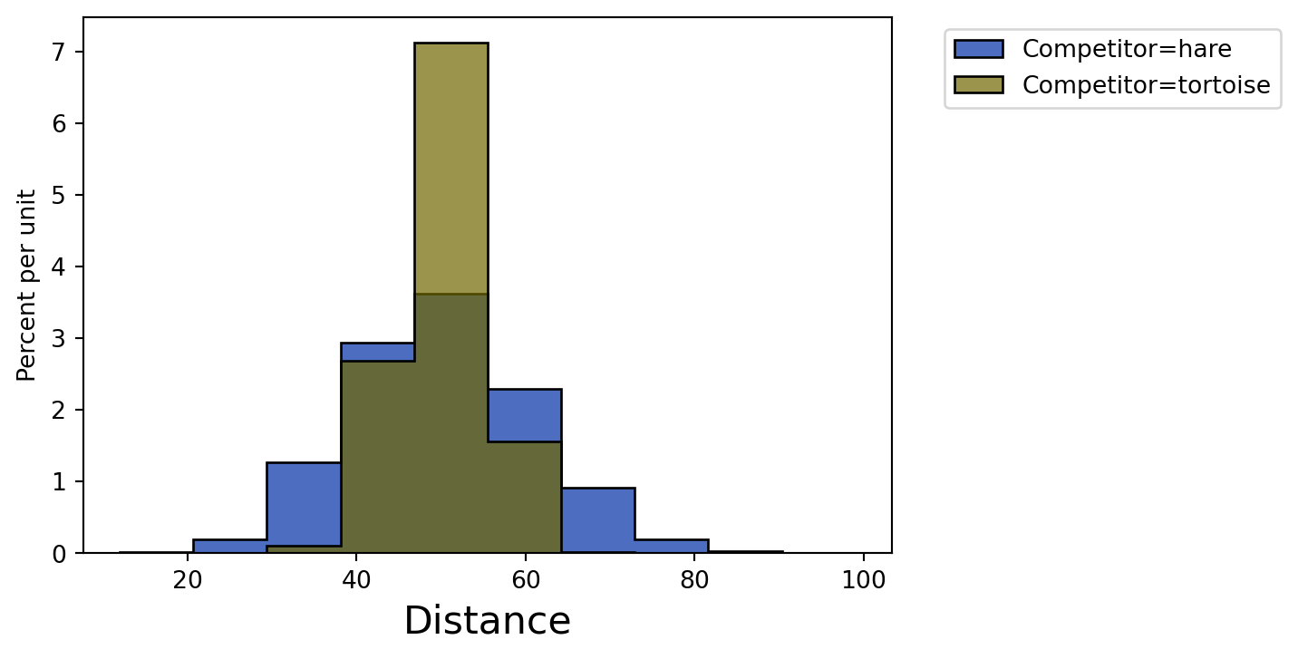
The results table (20,000 rows) contains two columns recorded after 10,000 simulations: - Competitor (string): the name of the competitor, either “tortoise” or “hare” - Distance (int): the final distance of the competitor at the end of the race
20.5.4 (d)
Using the results table, create an overlaid histogram that shows the distribution of final distances for both the tortoise and the hare.
Create an array called differences where each value in the array represents how many steps the hare finished ahead of the tortoise in a given race. Then, write a line of code to calculate the observed p-value of the hypothesis test. Finally, assuming a 5% p-value cutoff, describe the different conclusions you would come to based on the possible values of the observed p-value.
If the observed p-value is less than the 5% cutoff, we would consider this evidence against the null hypothesis and reject it in favor of the alternative hypothesis. If the observed p-value is greater than the 5% cutoff, our observation is consistent with our null hypothesis and we would fail to reject the null.
p_value
0.00029999999999999997
20.6 More Hypothesis Testing
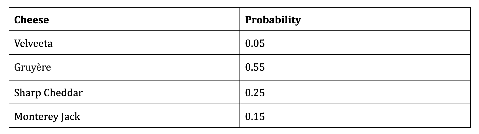
Chloe is a big fan of Trader Joe’s Frozen Mac ’n Cheese, but she noticed that the cheese used in it varies from box to box. A Trader Joe’s employee provides her with some data about the 4 different cheeses used and the probability of them being used in each box:
Chloe is suspicious about this distribution. After all, Velveeta is much cheaper to use than Gruyère, and she has also never bought a box that uses Gruyère. Chloe decides to buy many boxes throughout the next month and tracks the type of cheese used in each box. She uses this to conduct a hypothesis test.
20.6.1 (a)
Write a valid null and alternative hypothesis for this experiment.
Null Hypothesis:
Alternative Hypothesis:
AnswerNull Hypothesis: The types of cheese in the Frozen Mac ’n Cheese boxes are distributed according to the probability distribution provided by the employee. Any observed difference is simply due to chance. Alternative Hypothesis: The types of cheese in the Frozen Mac ’n Cheese boxes are not distributed according to the probability distribution provided by the employee. Any observed difference is not just due to chance.
The array observed_proportions contains the proportions of cheese that Chloe observed in 20 boxes of Mac ’n Cheese.
20.6.2 (b)
Chloe wants to use the mean as a test statistic, but Katherine suggests that Chloe use the TVD (total variation distance) instead. Which test statistic should Chloe use in this case? Briefly justify your answer. Then, write a line of code to assign the observed value of the test statistic to observed_stat.
Katherine is correct, we should use the total variation distance because she is comparing two categorical distributions (the observed distribution and the one provided by the Trader Joe’s employee).
Define the function one_simulated_test_stat to simulate a random sample according to the null hypothesis and return the test statistic for that sample.
Chloe simulates the test statistic 10,000 times and stores the results in an array called simulated_stats. The observed value of the test statistic is stored in observed_stat. Complete the code below so that it evaluates to the p-value of the test:
Given that the computed p-value is 0.0825, which of the following are true? Select all that may apply.
Answer
Only choice b is correct. We can only reject the null hypothesis when the observed p-value is less than the cutoff. Furthermore, there is no chance associated with whether or not the null or alternative hypothesis is true.
20.7 A/B Testing
NoteUnderstanding A/B Testing
Use an A/B test to check if two samples come from the same distribution.
In a permutation test, sample without replacement so that the proportions of categories stay the same when shuffling.
A permutation is just a reordering of the original data.
You can shuffle either the labels or the data column.
Remember: the p-value cutoff (like 0.05) represents the probability of falsely rejecting the null hypothesis — it is not the same as your observed p-value.
20.7.1 (a)
Kevin, a museum curator, has recently been given specimens of caddisflies collected from various parts of Northern California. The scientists who collected the caddisflies think that caddisflies collected at higher altitudes tend to be bigger. They tell him that the average length of the 560 caddisflies collected at high elevation is 14mm, while the average length of the 450 caddisflies collected from a slightly lower elevation is 12mm. He is not sure that this difference really matters and thinks that this could just be the result of chance in sampling.
What is an appropriate null hypothesis that Kevin can simulate under?
Answer
Null Hypothesis: The distribution of specimen lengths is the same for caddisflies sampled from high elevation as those sampled from low elevation. Any observed difference between the two samples is simply due to random chance.
20.7.2 (b)
How could you test the null hypothesis in the A/B test from above? What assumption would you make to test the hypothesis, and how would you simulate under that assumption?
Answer
If the null hypothesis is true – the caddisflies did not come from different distributions – then it should not matter how the samples were labeled (high elevation or low elevation). Under this assumption, you could shuffle the labels of the caddisflies and calculate your test statistic from this “relabeled” data.
20.7.3 (c)
What would be a useful test statistic for the A/B test? Remember that the direction of your test statistic should come from the initial setting.
Answer
Difference in mean lengths between the two groups. Note that this is not an absolute difference – we could choose either order for subtraction, but that would affect the direction of our alternative hypothesis so we need to be careful!
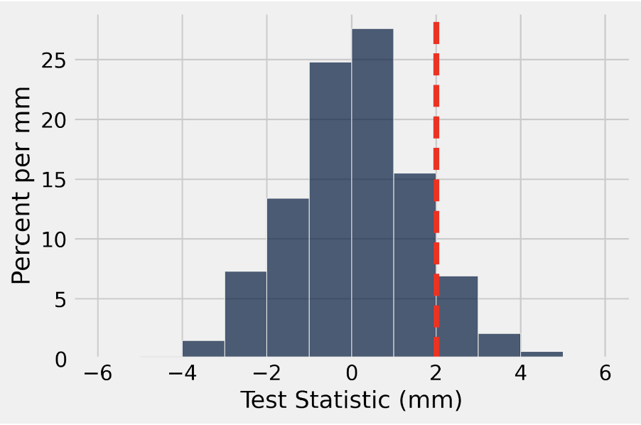
The histogram of test_stats is plotted below with a vertical red line indicating the observed value of our test statistic. If the p-value cutoff we use is 5%, what is the conclusion of our test?
Answer
We can inspect the histogram above to see that the area to the right of the observed value (which is our p-value) is greater than 5%. Since our p-value is greater than our p-value cutoff, we fail to reject the null hypothesis and conclude that the data tend to favor the null hypothesis.
20.7.7 (g)
Suppose that the null hypothesis is true. If we ran this same hypothesis test 1000 times, each time from our flies table and with a p-value cutoff of 5%, how many times would we expect to incorrectly reject the null hypothesis?
Answer
We would expect to reject the null hypothesis \(1000 * 0.05 = 50\) times. A p-value cutoff of 5% represents the probability of incorrectly rejecting the null hypothesis.
20.7.8 (h)
What effect does decreasing our p-value cutoff have on the number of times we expect to incorrectly reject the null hypothesis?
Answer
If we decrease our p-value cutoff, we are reducing the expected number of times we will incorrectly reject the null.
20.7.9 (i)
Answer the following True/False questions.
20.7.9.1 (i)
A/B testing is used to determine whether or not we believe two samples come from the same underlying distribution.
Answer
True, this is the definition of A/B testing.
20.7.9.2 (ii)
To conduct a permutation test, you should sample your data with replacement with a sample size equal to the number of rows in the original table.
Answer
False, you should sample your data without replacement–otherwise, you would not get a permutation of your data.
20.7.9.3 (iii)
A/B testing is the same as using total variation distance as a test statistic for a hypothesis test.
Answer
False, total variation distance is just a test statistic that computes the distance between two distributions. It does not involve taking a random permutation of your data.
20.8 Functions (Bonus!)
Cyrus loves completing the NYT Monday crossword puzzle, and is interested in seeing how fast he completes it in comparison with his friends. Over the past two months, Cyrus and his friend Monica have been recording their crossword completion times (in seconds) in the arrays cyrus_times and monica_times respectively. Cyrus decides to put his skills to the test by randomly selecting one of his times and comparing it to a randomly chosen time of Monica’s.
This type of problem might look like hypothesis testing, but the focus is on functions and string manipulation.
Example: one_comparison returns True/False, so it can be used directly in a conditional.
If a function only prints and doesn’t return, you can’t save its result in a variable.
Don’t forget to convert numbers to strings (like wins and trials) before concatenating them.
20.8.1 (a)
Write a function called one_comparison that randomly chooses one time from cyrus_times and one time from monica_times, and returns True if Cyrus’s time was better than Monica’s.
Now, write a function called crossword_comparison that takes in trials, which is the number of times we randomly compare one of Cyrus’s completion times with one of Monica’s. The function should print a statement explaining the total number of times Cyrus won. For example, if Cyrus won 6 times out of 10 trials, the statement should read “Cyrus beat Monica 6 times out of 10 trials”.
def crossword_comparison(trials): wins = ________for i in ________:if ________: wins = ________print("Cyrus beat Monica "+ ________ +" times out of "+ ________ +" trials")
Answer
def crossword_comparison(trials): wins =0for i in np.arange(trials):if one_comparison(): wins = wins +1print("Cyrus beat Monica "+str(wins) +" times out of "+str(trials) +" trials")
crossword_comparison(100)
Cyrus beat Monica 99 times out of 100 trials
20.8.3 (c)
Cyrus is interested in using his new function to show Monica that he is superior in crossword solving. He runs crossword_comparison over 100 trials, and assigns the output to a variable called my_wins for easy access. What is one issue with this process?
Answer
This function prints a sentence rather than returning a value or string. The variable my_wins will therefore be assigned to nothing, and could result in an error if it were to be used in any calculations.
print(crossword_comparison(100))
Cyrus beat Monica 100 times out of 100 trials
None
20.8.4 (d)
Finally, Cyrus wants to create a team of Data 8 course staff for competitive crossword-puzzle solving. However, he is particular and will only accept them if they satisfy the following two conditions:
He wants to create a very strong team, so He only wants to recruit people who have an average crossword completion time below 5 minutes.
He favorite number is 10, so of the people above he will only recruit those who have a last name that is exactly 10 letters long.
Write a function that takes in a table with three columns:
First (str): Player’s first name
Last (str): Player’s last name
Time (int): Player’s completion time for that puzzle in seconds
and returns an array of player names (First and Last) that Cyrus will recruit for his team. If Bing Concepcion is supposed to be in the array, you may leave his name as “BingConcepcion”.