from datascience import *19 Discussion 07: Assessing Models (from Fall 2025)
19.0.1 Contact Information
| Name | Wesley Zheng |
| Pronouns | He/him/his |
| wzheng0302@berkeley.edu | |
| Discussion | Wednesdays, 12–2 PM @ Etcheverry 3105 |
| Office Hours | Tuesdays/Thursdays, 2–3 PM @ Warren Hall 101 |
Contact me by email at ease — I typically respond within a day or so!
19.0.2 Announcements
When we observe something different from what we expect in real life (i.e., four 3’s in six rolls of a fair die), a natural question to ask is “Was this unexpected behavior due to random chance, or something else?”
Hypothesis testing allows us to answer the above question in a scientific and consistent manner, using the power of computation and statistics to conduct simulations and draw conclusions from our data.
19.1 Test Statistics
Dylan is playing with a coin and he wants to test whether his coin is fair. His experiment is to toss the coin 100 times. He chooses the following null hypothesis.
Null Hypothesis: The coin is fair and any observed deviation is due to chance.
For each of the alternative hypotheses listed below, determine whether or not the test statistic is valid and give an explanation.
19.1.1 (a)
Alternative Hypothesis: The coin is biased towards heads.
Test Statistic: # of heads.
Answer
19.1.2 (b)
Alternative Hypothesis: The coin is not fair.
Test Statistic: # of heads.
Answer
19.1.3 (c)
Alternative Hypothesis: The coin is not fair.
Test Statistic: \(|\)# of heads - expected # of heads \(|\).
Answer
19.1.4 (d)
Alternative Hypothesis: The coin is biased towards heads.
Test Statistic: \(|\)# of heads - expected # of heads \(|\).
Answer
This is the opposite case of part (b). We see that this test statistic will also account for a bias towards tails (because of the absolute value).
19.1.5 (e)
Alternative Hypothesis: The coin is not fair.
Test Statistic: \(\frac{1}{2}\) - proportion of heads.
Answer
19.2 Carnival Games
You are playing a wheel-spinning game at a carnival, where you can earn prizes based on where the wheel stops. The booth attendant claims the distribution of prizes is as below, but you think the game is rigged and doesn’t follow the listed probabilities.
| Prize | Chance |
|---|---|
| Nothing | 80% |
| Teddy bear | 2% |
| Pinwheel | 6% |
| Sticker | 12% |
You would like to test your claim so you can report the carnival for fraud.
19.2.1 (a)
Is the data we are working with numerical or categorical? Think about how this influences what test statistic we should use.
Answer
19.2.2 (b)
What is the booth attendant’s hypothesis?
Answer
The distribution of prizes follows the distribution listed by the carnival. Any observed difference is simply due to chance.19.2.3 (c)
What is your hypothesis?
Answer
The distribution of prizes does not follow the distribution listed by the carnival. Any observed difference is not just due to chance.19.2.4 (d)
Which hypothesis (of the two we defined) can you simulate under?
Answer
You could simulate under the booth attendant’s hypothesis. This is because it is a fully defined model, meaning we are able to describe the parameters of an experiment surrounding it. Your hypothesis is simply that the distribution is not the same as the carnival’s; there is no fully defined model that we can simulate under.19.2.5 (e)
What is a good statistic to use?
Answer
TVD from expected distribution. When we are observing categorical distributions of data and want to compare them, we should use TVD. Note, this is a good example because we have four different components in the distribution that we would like to test.19.2.6 (f)
Write code that simulates playing the carnival game 1000 times, and returns an array of proportions corresponding to how often each prize was won.
prize_chances = _______________________________________________________
my_simulation = _______________________________________________________
Answer
prize_chances = make_array(0.8, 0.02, 0.06, 0.12)
my_simulation = sample_proportions(1000, prize_chances)19.2.7 (g)
Write one line of additional code that extracts the number of teddy bears we would have won in our simulation. You may use my_simulation from the previous question.
Answer
my_simulation.item(1) * 100018.0Suppose the wheel-spinning game received a lot of complaints at the carnival, and the owners of the game are pressured to release their true distribution of prizes as below:
| Prize | Chance |
|---|---|
| Nothing | 90% |
| Teddy bear | 1% |
| Pinwheel | 3% |
| Sticker | 6% |
Use the distribution above to answer the following probability questions.
19.2.8 (a)
What is the probability of winning a prize from one spin of the wheel?
Answer
Using the Complement Rule:
\[P(winning\:a\:prize) = 1 -[winning\:a\:prize] = 1 − P[Nothing] = 1 − 0.9 = 0.1\:or\:10\%\]19.2.9 (b)
What is the probability of winning a Teddy bear and a Sticker in two spins?
Answer
\[P(Teddy\:bear\:and\:Sticker) = 2 * P(Teddy\:bear) * P(Sticker) = 2 * 0.01 * 0.06 = 0.12%\]
We multiply by 2 because we could have won the Teddy bear and then the Sticker OR the Sticker first and then the Teddy bear.
19.2.10 (c)
What is the probability of winning at least one prize in 10 spins?
Answer
Complement Rule again:
\[P(at\:least\:one\:prize) = 1 - P(no\:prizes\:in\:10\:spins) = 1 - P(Nothing) ^{10} = 1 - (0.9)^{10}\]19.3 Flu (Bonus!)
Researchers are studying the effectiveness of a particular flu vaccine. A large random sample was taken from the population of people who took the vaccine in 2016. Among the sampled people, 48% did not get the flu. Another large random sample was taken in 2017, from among the people who took the vaccine that year. Among these sampled people, 40% did not get the flu.
(Spring 2018 Midterm Question 4)
19.3.1 (a)
A researcher thinks the vaccine was less effective in 2017 than in 2016. To test this, a null hypothesis is needed. Which is the correct null hypothesis?
Answer
Option A - Incorrect as it describes a model that is difficult to simulate under. How can we quantify “less effective”?
Option B - Incorrect as the question tells us that the vaccine was not equally effective in the two samples (48% vs 40%).
Option C - Correct. The null hypothesis would state that the vaccine was equally effective in the two populations, and that the differences we observe in the two samples are simply due to chance.
19.3.2 (b)
The researcher says, “The observed value of my test statistic is \(40\% - 48\% = − 8\%\).” To perform the test, the statistic is simulated under the null hypothesis. One of the figures below is the empirical histogram of the simulated values. Which is it?
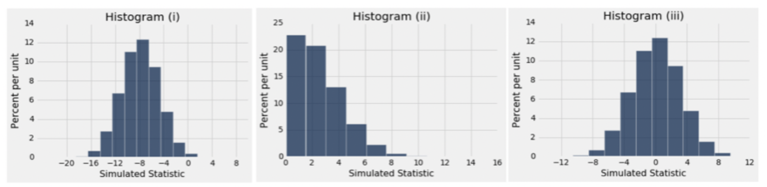
Answer
The test statistic we are using is the difference between the two sample percentages. Under the null hypothesis, this could be positive or negative depending on the sample. This rules out (ii).
Under the null hypothesis, the two sample percentages are expected to be equal and hence the difference is expected to be 0. This rules out (i).
Only (iii) has all the right properties.