16 Discussion 14: MLR & Bayes (from Fall 2025)

16.0.1 Contact Information

Name	Wesley Zheng
Pronouns	He/him/his
Email	wzheng0302@berkeley.edu
Discussion	Wednesdays, 12–2 PM @ Etcheverry 3105
Office Hours	Tuesdays/Thursdays, 2–3 PM @ Warren Hall 101

Contact me by email at ease — I typically respond within a day or so!

16.0.2 Announcements

Announcements

Please remember to complete your course evaluations — your feedback matters!
Important: If you have not interacted with a GSI, please do not provide feedback or ratings for them.

16.1 Multiple Linear Regression

In multiple linear regression, a numerical output is predicted from multiple attributes; the output is obtained by multiplying each attribute value by a different slope and then summing the results. Much like simple linear regression, we will find our optimal slopes by minimizing the root mean squared error (RMSE) between our actual values and our predicted values.

Below is a table rides that contains data on 1000 theme park rides. There are three columns:

Number of Visitors (int): the total number of visitors currently in the entire theme park.
Popularity Score (int): a rating from 0 to 100 measuring how popular the ride is.
Wait Time (int): the average wait time for the ride in minutes.

Code

from datascience import *
import numpy as np

fixed_visitors = [400, 700, 1100, 1500, 1800]
fixed_popularity = [30, 50, 75, 85, 90]
fixed_wait = [20, 35, 55, 70, 80]

n_remaining = 995
visitors_rest = np.random.randint(100, 5000, size=n_remaining)
popularity_rest = np.random.randint(0, 101, size=n_remaining)
noise_rest = np.random.normal(0, 5, size=n_remaining)
wait_rest = 0.015 * visitors_rest + 0.5 * popularity_rest + noise_rest
wait_rest = np.round(wait_rest).astype(int)

visitors_all = fixed_visitors + visitors_rest.tolist()
popularity_all = fixed_popularity + popularity_rest.tolist()
wait_all = fixed_wait + wait_rest.tolist()

rides = Table().with_columns(
    "Number of Visitors", visitors_all,
    "Popularity Score", popularity_all,
    "Wait Time", wait_all
)

rides.show(5)

train = rides.take(np.arange(750))
test = rides.take(np.arange(750, 1000))

Number of Visitors	Popularity Score	Wait Time
400	30	20
700	50	35
1100	75	55
1500	85	70
1800	90	80

... (995 rows omitted)

SangJun is interested in predicting the average wait time of a ride, measured in minutes, given the Number of Visitors and Popularity Score attributes.

16.1.1 (a)

Assume SangJun has determined that MLR is a good model choice, and has correctly split the data into a test and train table. Help SangJun define a function predict(slope1, slope2, intercept, tbl) that takes in two slopes, an intercept, and a table with the same structure as rides and predicts the wait times for all rows in the table. Assume that the first column in the table corresponds to slope1, and the second column corresponds to slope2.

def predict(slope1, slope2, intercept, tbl):
  ______________________________________________

Answer

def predict(slope1, slope2, intercept, tbl):
    return slope1 * tbl.column(0) + slope2 * tbl.column(1) + intercept

predict(0.02, 0.4, 5, train)

array([  25.  ,   39.  ,   57.  ,   69.  ,   77.  ,   29.36,   41.62,
         66.34,   91.9 ,   79.34,   25.1 ,   97.92,   59.74,  101.52,
         40.68,   59.6 ,  130.78,  110.26,   26.1 ,  106.34,   84.98,
        115.74,  100.48,  107.34,  108.78,   31.62,   48.68,   50.82,
        120.36,   58.22,   95.94,   94.24,   49.18,   39.5 ,  121.82,
         93.86,  127.74,   69.88,  100.5 ,   60.72,   65.9 ,   49.9 ,
         76.64,   22.04,  101.26,  143.56,   75.04,   85.68,   79.  ,
         49.56,   31.28,   57.38,   97.68,   83.4 ,   55.74,   59.04,
        106.22,   47.48,   52.56,   32.98,   88.24,   80.8 ,   39.44,
         59.2 ,   60.08,   48.46,  119.9 ,  113.14,  102.68,   94.28,
        103.86,   71.64,   94.86,   32.64,   99.98,   79.18,  121.66,
        111.38,   42.78,   80.14,   49.26,  107.16,   71.22,   66.36,
         82.26,   31.98,   13.66,   41.48,   32.7 ,   62.02,   27.26,
        128.02,  111.06,   43.7 ,   35.86,   74.46,   71.68,  100.62,
         11.6 ,   58.  ,  130.34,   18.68,  108.52,  105.98,  107.4 ,
         47.14,  102.52,   64.98,   96.26,   40.58,  107.36,   72.92,
        131.74,   77.12,   24.52,   99.14,   42.68,   39.68,  107.3 ,
         88.82,   63.08,  103.16,  137.8 ,   19.02,   41.9 ,   34.28,
        138.04,  106.78,   97.12,   58.98,  109.24,   92.8 ,   82.62,
         94.4 ,  102.36,   86.46,  100.32,   88.22,   89.8 ,   35.86,
        108.24,  117.98,  106.56,   96.62,   56.32,   32.6 ,   65.56,
         76.02,   92.54,   88.16,  113.34,  108.14,   60.54,   98.28,
         62.12,   56.32,   49.24,   47.54,   54.34,   90.78,   80.62,
         62.96,   55.94,  113.92,   76.52,  128.12,  104.4 ,   90.8 ,
         99.8 ,  105.42,  123.2 ,   68.66,   82.88,  123.34,   61.9 ,
         30.42,   32.44,   82.44,   56.96,   88.3 ,   80.74,  101.2 ,
        103.1 ,   35.14,  118.16,   19.08,   71.56,   39.24,   80.08,
         62.08,   27.64,   81.34,    7.04,   97.68,   87.1 ,  103.26,
         62.14,   95.26,  119.96,  107.94,   49.62,   86.06,   78.84,
        104.8 ,   40.6 ,   43.64,   74.04,  114.44,   43.6 ,   48.14,
         83.38,  106.56,  109.26,  137.02,   91.38,   18.74,   92.22,
         18.04,   76.68,   21.16,   76.32,   56.18,   41.86,   65.06,
        104.98,   51.8 ,   78.08,  132.84,  111.12,  100.18,   66.72,
         95.46,  136.02,   85.28,  119.32,  114.78,   67.32,   53.32,
        134.8 ,   69.9 ,   78.42,   35.54,   98.02,  109.68,   49.64,
        120.72,  126.32,  105.48,   70.44,   66.8 ,   44.3 ,  122.64,
         38.6 ,  102.76,   63.16,  106.84,   82.58,   95.18,  104.92,
         69.08,   53.34,  105.1 ,   64.64,   80.26,   64.82,   58.3 ,
         42.44,   59.52,   29.48,   59.64,   49.82,  119.5 ,   37.96,
         96.84,   74.92,   74.06,   85.48,  100.96,   98.78,   86.22,
         49.94,   75.34,  108.34,  124.08,   84.34,   99.26,  111.  ,
         47.96,   59.74,  106.98,  118.84,   46.96,   50.14,  120.7 ,
        131.14,   65.14,  117.06,   88.  ,   68.24,   58.38,   74.  ,
         85.4 ,  101.18,   48.62,   72.04,  120.1 ,   60.32,  120.16,
         17.74,   81.04,   71.26,   56.1 ,   94.66,   70.88,   82.56,
         71.58,   88.88,   52.1 ,   88.98,   52.54,   61.8 ,   35.46,
         39.7 ,   70.62,   73.54,   58.82,   40.94,   70.8 ,  133.36,
         44.3 ,   80.54,   53.92,   61.08,  109.42,  108.12,   35.04,
         72.9 ,   60.2 ,   20.82,   77.34,   90.32,  102.96,   47.04,
         50.78,   63.52,  109.02,   90.02,   88.4 ,   91.3 ,   50.52,
        121.68,   85.56,   94.32,   74.08,   73.62,   65.66,   25.26,
        100.12,   45.62,  104.9 ,   48.46,   17.88,   29.72,  113.06,
         74.54,   41.44,   66.56,   93.18,   91.28,  113.6 ,   25.08,
        110.74,  106.66,   73.68,   38.42,   87.38,  123.96,   67.02,
         66.88,   83.42,   46.96,   97.62,   49.18,   76.86,  126.32,
         26.06,  129.58,   77.48,   52.16,  115.78,  132.34,  111.02,
        119.04,   73.4 ,   52.08,   55.08,   78.46,  124.02,   81.12,
         62.86,   89.3 ,   71.04,   92.82,  101.86,   74.9 ,   86.52,
         70.96,  108.24,   74.  ,   58.6 ,   22.8 ,   28.9 ,   75.74,
         55.84,   39.18,   31.56,   90.1 ,   98.36,   15.64,  110.92,
         92.92,   83.38,   35.36,   60.98,   53.12,  103.78,   30.32,
         40.46,   98.02,   76.76,  125.02,   80.06,  108.44,   42.32,
         56.56,   98.28,   67.5 ,   59.74,  122.18,   12.98,  104.08,
         97.42,   21.32,   57.  ,   62.86,   44.54,   82.5 ,   30.02,
         76.9 ,   72.36,  105.26,   58.82,   95.52,   19.54,   29.96,
         68.7 ,   86.9 ,   53.34,  130.54,   33.8 ,   48.58,   87.56,
        127.26,   87.1 ,   59.74,   73.36,   32.88,   77.48,   26.48,
         56.62,   39.42,   72.44,   98.34,   54.5 ,   68.22,   41.98,
        104.64,   62.76,   38.88,   44.94,   24.04,  109.3 ,   68.44,
         39.26,   42.86,   83.44,   55.54,   22.74,  100.74,   34.12,
         65.74,   78.32,  101.06,   50.62,   44.58,   73.8 ,   47.44,
         13.06,   17.66,  114.6 ,   80.76,   59.28,   64.08,   32.74,
        110.24,   45.52,   40.76,   78.9 ,   71.62,  100.98,   25.76,
         54.52,  104.92,   82.96,   85.96,   77.98,   85.88,   36.24,
        101.42,   93.66,  116.14,   98.34,   75.34,   79.9 ,  106.5 ,
        121.3 ,   79.8 ,   94.38,   45.46,   60.22,   55.36,   50.48,
         96.16,   77.82,  141.92,  131.92,   54.18,  109.8 ,   63.48,
        140.46,   52.84,   49.98,  109.24,   86.76,   35.4 ,  131.78,
         67.  ,  117.88,   65.16,  109.7 ,   66.52,  112.52,   25.76,
         25.46,  105.42,   92.4 ,  102.98,   47.42,   53.54,  129.94,
         54.68,  144.48,  107.92,  102.66,  103.24,   93.68,   94.86,
        105.02,   71.36,  120.14,   26.68,  108.44,  140.06,   42.46,
        129.58,   43.12,  114.68,  105.38,  115.16,   62.26,   42.08,
        100.4 ,   10.56,  127.74,   76.88,   98.32,  108.  ,   57.74,
         87.24,   57.98,   68.1 ,   80.28,   28.22,   89.8 ,   12.4 ,
         80.34,  103.68,   40.88,  119.38,   40.64,   96.06,   32.06,
         81.22,   71.14,  108.  ,  104.8 ,   71.58,   69.62,   74.38,
        131.  ,   55.34,   43.02,   43.46,   40.24,   61.24,   85.28,
        123.14,   69.42,   99.3 ,   41.  ,  107.44,   73.98,   45.92,
         93.54,   28.7 ,   85.  ,  107.52,   54.44,   80.94,   23.44,
         34.96,  104.1 ,   47.62,   91.04,   36.48,   89.12,   47.18,
         59.06,   82.18,  107.12,   91.2 ,   66.86,   42.6 ,   18.56,
         65.72,  136.06,  113.6 ,   41.44,   48.86,   29.2 ,  115.34,
         17.08,   62.66,   90.9 ,   89.78,   21.36,   93.28,   57.92,
         54.62,   44.58,   61.12,   72.8 ,   46.84,   90.48,   64.34,
        111.08,   52.74,  106.64,  142.16,   46.02,   28.28,   73.88,
         98.28,  130.26,   75.54,   45.16,   91.34,  113.66,   42.78,
         85.86,   77.58,   57.84,   72.06,   52.58,   48.28,   51.5 ,
         56.96,  132.3 ,  130.8 ,   48.4 ,   50.04,  103.6 ,   39.58,
        100.46,   95.86,   73.76,   82.74,   85.76,   99.26,   53.08,
         91.82,   42.06,  125.04,   83.9 ,   96.96,   99.78,  118.22,
         87.5 ,   58.48,   33.14,   92.54,  122.04,   76.1 ,   51.04,
        112.54,   36.12,   84.72,  110.32,   95.64,   97.1 ,   58.94,
        113.28,   65.06,   81.7 ,  115.5 ,   26.98,  112.28,   46.5 ,
        118.24,  103.82,   79.3 ,   63.14,   76.8 ,   82.84,   85.7 ,
         75.08,   45.8 ,  102.36,   58.98,   77.92,   68.98,   48.76,
         80.14,  101.02,   60.68,  110.7 ,  113.04,   35.66,   73.6 ,
         27.56])

16.1.2 (b)

Using the predict function, help complete the code for the function train_rmse(slope1, slope2, intercept) that takes in two slopes and an intercept and computes the RMSE of the predictions on the train table:

def train_rmse(slope1, slope2, intercept):
  predictions = ________________________________________
  actual = __________________________________________
  residuals = _________________________________________
  _________________________________________

Answer

def train_rmse(slope1, slope2, intercept):
    predictions = predict(slope1, slope2, intercept, train)
    actual = train.column("Wait Time")
    residuals = actual - predictions
    return np.sqrt(np.mean(residuals ** 2))

train_rmse(0.02, 0.4, 5)

15.190575271090516

16.1.3 (c)

Assume that after following the demos from lecture, SangJun has properly defined the train_rmse(slope1, slope2, intercept)} function and assigns best_slopes to the result of calling

minimize(train_rmse, start= make_array(5, 5, 5), smooth=True, array=True)

Assume the array best_slopes evaluates to array([0.02, 0.4, 5]). Help SangJun answer the following questions about his results.

16.1.3.1 (i)

Write out the equation of the regression line as a mathematical expression, using the values in best_slopes.

Answer

\(\text{Predicted Wait Time} = 0.02 * \text{Number of Visitors} + 0.4 * \text{Popularity Score} + 5\)

16.1.3.2 (ii)

Using the equation above, what would the predicted wait time be for a ride when there are 1000 visitors currently in the park and the ride has a popularity score of 70?

Answer

\[ \begin{aligned} \text{Predicted Wait Time} &= 0.02 \times \text{Number of Visitors} + 0.4 \times \text{Popularity Score} + 5 \\ &= 0.02 \times 1000 + 0.4 \times 70 + 5 \\ &= 20 + 28 + 5 \\ &= 53 \end{aligned} \]

So, the predicted wait time is 53 minutes.

16.1.4 (d)

How would we interpret the slope for the “Number of Visitors” attribute? Write your answer in 1-2 sentences, making sure to use precise language.

Answer

The slope for the Number of Visitors attribute is 0.02. This means that for every additional visitor in the park, the predicted wait time increases by 0.02 minutes, holding all other variables constant.

Interpreting the Meaning of a Regression Slope

The slope in regression tells you how much the predicted outcome changes when your input variable increases by one unit, assuming all other variables stay the same. Be precise with this interpretation because it helps understand model results clearly.

16.2 Thomas’ Bays

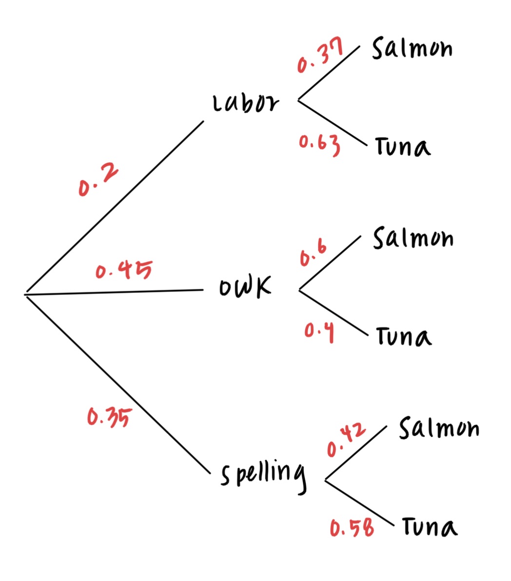
Thomas is an avid consumer of fish and is interested in finding ethically sourced fish to eat from 3 local bays near him. He researches online and finds the following information:

Out of all fish, \(20\%\) of fish come from Labor Bay, \(45\%\) of fish come from Obi-Wan Keno Bay, and \(35\%\) come from Spelling Bay.
In these three bays, there are only 2 types of fish: salmon and tuna.
In Labor Bay, \(37\%\) of the fish are salmon.
In Obi-Wan Keno Bay, \(40\%\) of the fish are tuna.
In Spelling Bay, \(42\%\) of the fish are salmon.

16.2.1 (a)

Draw a tree diagram to represent the result of Thomas’ research.

Understanding Probability Trees: Visualizing Compound Events

Probability trees are great tools to map out all possible outcomes step-by-step. At every split in the tree, the probabilities of all branches add up to 1. For example, imagine a bag containing two dice: one is weighted to roll a 6 half the time, the other is a normal die. You randomly pick one (50-50 chance), then roll it. The tree helps you see the total probability of rolling a six by multiplying the chance of picking a die by the chance of rolling six on that die.

Answer

16.2.2 (b)

Thomas is shopping for a fish at random. What is the chance he picks a tuna from Obi-Wan Keno Bay?

Answer

\(P(\text{Tuna and Obi-Wan Keno Bay}) = P(\text{Tuna} \mid \text{OWK}) \cdot P(\text{OWK}) = 0.4 \times 0.45\)

Using the Multiplication Rule to Calculate Combined Probabilities

To find the probability of multiple events happening together, multiply the probabilities along the branches of the probability tree that lead to the event. You can trace the branches to understand how combined probabilities work. This helps you see complex event chances clearly.

16.2.3 (c)

Thomas chooses a fish at random.

16.2.3.1 i.

What is the probability that the fish is a salmon?

Answer

\(P(\text{Salmon}) = 0.2 \cdot 0.37 + 0.45 \cdot 0.6 + 0.35 \cdot 0.42 = 0.491\)

16.2.3.2 ii.

What is the probability that it is a tuna?

Answer

\(P(\text{Tuna}) = 0.2 \cdot 0.63 + 0.45 \cdot 0.4 + 0.35 \cdot 0.58 = 0.509\)

or we can compute the complement of the part (i) which gives

\(P(\text{Tuna}) = 1 - P(\text{Salmon}) = 0.509\)

Marginal Probability: Finding the Overall Chance of an Event

Marginal probability means the total chance of an event happening, regardless of other conditions. For example, if you want the chance of getting a salmon, add up the probabilities of all the different ways you could get salmon. You can also find the chance of getting tuna as the complement (everything else), like:

\(P(\text{Tuna}) = 1 - P(\text{Salmon})\)

You can also calculate tuna probability directly by adding the relevant branches.

16.2.4 (d)

Thomas ends up buying a salmon. What is the probability the salmon came from Spelling Bay?

Answer

\[ \begin{aligned} P(\text{Spelling Bay} \mid \text{Salmon}) &= \frac{P(\text{Spelling Bay and Salmon})}{P(\text{Salmon})} \\ &= \frac{0.35 \cdot 0.42}{0.2 \cdot 0.37 + 0.45 \cdot 0.6 + 0.35 \cdot 0.42} \end{aligned} \]

Applying Bayes’ Rule with Probability Trees

Bayes’ Rule helps us update probabilities when given new information. The denominator in Bayes’ formula is the total probability of the condition (like Thomas buying a salmon), which you get by adding all the relevant salmon branches on the tree. The numerator is the joint probability of both events happening (like Thomas buying a salmon from Spelling Bay). Divide numerator by denominator to get the conditional probability:

\(P(\text{Spelling Bay} | \text{Salmon}) = \frac{P(\text{Spelling Bay and Salmon})}{P(\text{Salmon})}\)

You can circle the relevant parts on the tree to visualize the numerator and denominator, which makes it easier to understand.

16.2.5 (e)

Thomas buys 10 fish at random. What is the probability that at least one of them is a salmon from Spelling Bay?

Answer

\[ \begin{aligned} P(\text{Salmon from Spelling Bay}) &= 0.35 \times 0.42 \\ P(\text{Salmon not from Spelling Bay}) &= 1 - (0.35 \times 0.42) \\ P(\text{Salmon not from Spelling Bay for all 10 times}) &= 1 - P(\text{Salmon not from Spelling Bay})^{10} = \left( 1 - (0.35 \times 0.42) \right)^{10}\\ P(\text{At least one salmon from Spelling Bay}) &= 1 - \left( 1 - (0.35 \times 0.42) \right)^{10} \end{aligned} \]

Solving “At Least One” Probability Problems with Complements

These problems often require careful use of the complement rule. For example, the probability that at least one salmon comes from Spelling Bay is NOT the same as the probability that a salmon is from Spelling Bay given it’s salmon. Use the complement rule twice: find the chance that none satisfy the condition, then subtract from 1 to get the “at least one” probability.

16.3 Blackboard Erasers

(Fall 2020 Final, Q3)

Mr. White is a teaching Chemistry class in Latimer Hall. His class has 100 undergraduate staff (uGSIs, tutors, etc.). Mr. White learns that one of his staff is stealing blackboard erasers from his lecture hall when the building is closed overnight. The only way the thief could access the building overnight is with a key card that belongs to them.

Suppose Mr. White discovers that 10 of his staff have a key card.

16.3.1 (a)

If Mr. White randomly selects one of his staff, what is the probability that they are the eraser thief?

Answer

0.01. Mr. White has 100 staff members, and 1 of them is the thief, so \(\frac{1}{100} = 0.01\)

16.3.2 (b)

If Mr. White randomly selects one of his staff, what is the probability that they are not the eraser thief and has a key card?

Answer

\(0.99 \cdot \frac9{9}{99}\). 99 out of 100 staff are not the thief. Since the thief has the key card as well, we account for probability.

\(P(\text{not eraser thief and has key card}) = P(\text{has key card} \mid \text{not eraser thief}) \cdot P(\text{not eraser thief}) = \frac{9}{99} \cdot 0.99\)

16.3.3 (c)

At the next course staff meeting, Mr. White notices that one of his GSIs, Gus, has a key card sticking out of his wallet. Given this information, what is the probability that Gus is the eraser thief?

Answer

We want to compute \(P(\text{Gus is the thief} \mid \text{Gus has a key card})\) using Bayes’ Rule, since the provided information was that Gus has a key card.

\[ \begin{aligned} P(\text{Gus is the thief} \mid \text{Gus has a key card}) &= \frac{P(\text{Gus has a key card} \mid \text{Gus is the thief}) \cdot P(\text{Gus is the thief})} {P(\text{Gus has a key card})} \\[6pt] &= \frac{1 \cdot 0.01}{P(\text{Gus has a key card})} \end{aligned} \]

The probability that Gus has a key card can be decomposed into:

Gus is the thief and has a key card
Gus is not the thief and has a key card

Therefore,

\[ P(\text{Gus has a key card}) = 0.01 + 0.99 \cdot \frac{9}{99} \]

And so the final answer is:

\[ P(\text{Gus is the thief} \mid \text{Gus has a key card}) = \frac{1 \cdot 0.01}{0.01 + 0.99 \cdot \frac{9}{99}}. \]

16.3.4 (d)

Mr. White is skeptical of his head GSI, Jesse. Prior to learning any information about Jesse’s key card access, Mr. White believes there is a 25% probability that Jesse is the eraser thief.

Suppose Mr. White later discovers that Jesse has a key card. Given this new information, what is the probability that Jesse is the eraser thief?

How Changing Priors Affects Bayesian Posterior Probabilities

In Bayesian inference, changing the prior probability (like setting it to 25%) changes the posterior probabilities you calculate. The prior expresses your initial belief before seeing data, so adjusting it naturally changes your updated beliefs.

Answer

The prior is \(P(\text{Jesse is the thief}) = 0.25\) and we want to compute \(P(\text{Jesse is the thief} \mid \text{Jesse has a key card})\).

Like above, we compute this with Bayes, except that we now have an updated prior,

\[ \begin{aligned} \frac{P(\text{Jesse has a key card} \mid \text{Jesse is the thief}) \cdot P(\text{Jesse is the thief})} {P(\text{Jesse has a key card})} &= \frac{1 \cdot 0.25}{0.25 \cdot 1 + 0.75 \cdot \frac{9}{99}} \end{aligned} \]

16 Discussion 14: MLR & Bayes (from Fall 2025)

16.0.1 Contact Information

16.0.2 Announcements

16.1 Multiple Linear Regression

16.1.1 (a)

16.1.2 (b)

16.1.3 (c)

16.1.3.1 (i)

16.1.3.2 (ii)

16.1.4 (d)

16.1.5 (e)

16.1.5.1 i.

16.1.5.2 ii.

16.1.5.3 iii.

16.1.5.4 iv.

16.1.5.5 v.

16.2 Thomas’ Bays

16.2.1 (a)

16.2.2 (b)

16.2.3 (c)

16.2.3.1 i.

16.2.3.2 ii.

16.2.4 (d)

16.2.5 (e)

16.3 Blackboard Erasers

16.3.1 (a)

16.3.2 (b)

16.3.3 (c)

16.3.4 (d)