27 Discussion 15: Wrapping Up (Extra) (from Fall 2025)
27.1 Semester Recap (Extra)
Write or describe the appropriate concept from this class that would be applied (e.g., hypothesis test, linear regression, classification, etc.) to answer each of these questions surrounding data. If no method is applicable explain why. You might remember some examples from the very first worksheet!
27.1.1 (a)
Estimating the average amount of students in each class at UC Berkeley based on a random sample.
Answer
Perform bootstrap resamples from the original sample and construct a confidence interval.27.1.2 (b)
Predicting whether or not a customer will make an online purchase based on their browsing activity.
Answer
Classification — they will either make a purchase or they won’t. We could use features like the amount of items in their shopping cart, amount of time spent browsing, amount of searches/visits, etc.27.1.3 (c)
Updating the probability someone will make a purchase based on new information about their household income bracket.
Answer
We can apply the concepts of Bayes’ Rule to update the probability of making a purchase with new information.27.1.4 (d)
Determining if there is any difference in household utility bills between Massachusetts and California.
Answer
We can run a hypothesis test. Since we are comparing household utility bills in two distributions (Massachusetts and California), we can perform an A/B test and use a test statistic such as the differences in means.27.1.5 (e)
Predicting how many students will graduate in a particular major based on the amount of Reddit posts about the subject.
Answer
Linear regression. We can further use regression inference to determine whether or not an association exists between these two variables.27.1.6 (f)
Determining whether a random Data 8 student in Fall 2024 sleeps on their stomach assuming you have data on how every single Data 8 student sleeps.
Answer
Since we have the entire population data set there is no reason to make a prediction. Instead, we can just look up the student in the data set and see what their preference is!
27.2 Confidence Intervals - Fa20 Final Q6 Modified (Extra)
Every day, Samiksha gets a boba drink from Asha in Berkeley. She believes the machine that’s used to add the boba pearls to the drink is calibrated to put an exact amount of boba in each drink, with some variability due to chance.
To get a sense of how the amount of boba in a drink varies, Samiksha plans to randomly sample customers throughout November and record the weight (in grams) of the boba pearls in each customer’s drink.
27.2.1 (a)
Suppose that Samiksha wants to use a sample of size 100 to create a confidence interval for the true population mean of boba weight per drink.
Which of the following could be used to help her create this confidence interval? Select all that are correct:
- Central Limit Theorem
- Bootstrapping
- Nearest Neighbors
- Linear Regression
- Classification
Answer
A and B are correct.27.2.2 (b)
Suppose that Samiksha wants to use a sample of size 100 to create a confidence interval for the true population median of boba weight per drink.
Which of the following could be used to help her create this confidence interval? Select all that are correct:
- Central Limit Theorem
- Bootstrapping
- Nearest Neighbors
- Linear Regression
- Classification
Answer
Only B is correct. The CLT only applies to the sum or mean of a random sample, not the median.
27.2.3 (c)
Suppose that Samiksha observes an average of 30 grams of boba per drink from a random sample of 100 customers and she knows that the population SD is 2 grams.
Which of the following is guaranteed to be true? Select all that are correct:
- At least 68% of the customers in the population will have a boba weight that is between 2 grams below and 2 grams above the population mean.
- At least 75% of the customers in the population will have a boba weight that is between 4 grams below and 4 grams above the population mean.
- At least 75% of the customers in the population will have a boba weight that is between 26 grams and 34 grams.
- At least 68% of the customers in Samiksha’s sample have a boba weight that is between 28 grams and 32 grams.
Answer
Only B is correct. We do not know if the population is normally distributed, so we can only use Chebyshev’s bounds. Chebyshev’s bounds tell us that 75% of the data lies within 2 SDs of the mean.
27.2.4 (d)
Suppose that Samiksha samples 500 customers and her 95% confidence interval for the true population mean is (29, 31).
Which of the following can be concluded from this confidence interval? Select all that are correct:
- If Samiksha repeats this process 1000 times, she can expect that roughly 95% of the intervals she creates will contain the true population mean.
- If Samiksha gets boba once a day throughout November, she can expect to get between 29 and 31 grams of boba on roughly 95% of the days.
- If Samiksha gets boba once a day throughout the year, she can expect to get between 29 and 31 grams of boba on roughly 95% of the days.
- If you sample 100 Asha boba customers in November, you can expect roughly 95% of them to get between 29 and 31 grams of boba.
Answer
Only A is correct. B, C, and D are all incorrect as the confidence interval is estimating the true average grams of boba in drinks, and makes NO claim about what percentage of days have between 29 and 31 grams of boba. It wouldn’t make sense to think that 95% of drinks all have between 29 and 31 grams of boba - those bobaristas would have be super precise!
27.3 Variability of Sample Mean - Fa19 Final Q9 Modified (Extra)
Ethan, an International Relations major, is writing his Masters thesis on aid given to foreign governments by the World Bank. He finds a sample of donations given to various countries over the last decade and collects these findings into a table called . Here are the first few rows.
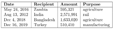
The table contains four columns:
- Date: a string, the date upon which the donation was made
- Recipient: a string, the country receiving the money
- Amount: an int, the amount of the donation in USD
- Purpose: a string, the reason listed for the aid
For parts (a) and (b), assume that Ethan is interested in studying the average Amount of aid given per donation.
27.3.1 (a)
To get a sense of the data, Ethan first plots a histogram of the aid ‘Amount’ in his sample. He finds that the empirical distribution of ‘Amount’ has an average of $3,532,423 and an SD of $1,121,240. The distribution of ‘Amount’ in his sample is:
- Approximately normal
- Not approximately normal
- There isn’t enough information to answer this question
Answer
C. There isn’t enough information to answer this question. We cannot tell whether Amount is normal based on the sample statistics given. It is definitely possible as 3 SDs in each direction is still a valid dollar amount.
27.3.2 (b)
Suppose Ethan wants to use his sample data to create a 95% confidence interval of the true average amount of aid of all donations. If the distribution of all World Bank donations has an SD of $1,000,000 and the aid table contains 10,000 rows, can Ethan create a 95% confidence interval that has a width less than $25,000?
Note: an interval of [-5, 5] has a width of 10.
- He can because the sample size is large enough
- He can’t because the sample size is too small
- There isn’t enough information to answer this question
Answer
B. He can’t because the sample size is too small. We’re given the sample size of 10,000 and the population SD of 1,000,000.
We can find the SD of the sample means to be \(\cfrac{1,000,000}{\sqrt{10,000}} = 10,000\).
Since we’re making a CI for the true average amount of aid, the CLT applies to the distribution of sample means. We know a 95% CI must have a width of 4 SDs. However, \(4 \cdot 10,000 > 25,000\), so the sample size is too small for such a narrow interval.For the rest of the question, assume that Ethan has turned his attention to learning more about aid ‘Purpose’.
27.3.3 (c)
As Ethan is combing through the data set, he notices that some countries in South Asia appear to have received a disproportionate amount of aid with the purpose of ‘rail’ and ‘manufacturing’ compared to others in the region. He creates the following table, which displays the aid given to countries in the region with the following proportions. For example, the last column tells us that of the aid that Pakistan received from the World Bank, 20% was for agriculture, 20% was for rail, and 60% was for manufacturing. Note that each country’s column adds up to 1.
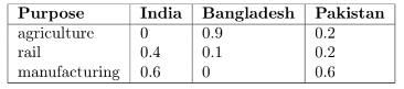
According to the above distributions, what is the empirical total variation distance of aid ‘Purpose’ between India and Bangladesh? You may leave your answer as a mathematical expression (not Python).
\[ \underline{\hspace{12cm}} \\ \]
Answer
We find the sum of the absolute differences between the corresponding purposes, and divide by 2. \(\cfrac{0.9 + 0.3 + 0.6}{2} = 0.9\).27.3.4 (d)
The World Bank claims the total variation distance of aid ‘Purpose’ between India and Bangladesh is 0.3. Ethan is not sure if his empirical TVD (from part (a)) is different from 0.3 just due to chance, but he thinks he could bootstrap his sample to get a better idea.
Complete the code below to write a function purpose_tvd that takes in a table tbl with the same column labels as aid, two country names, country_a and country_b, and computes the total variation distance between the two countries’ ‘Purpose’ distributions.
For example, purpose_tvd(aid, ‘Bangladesh’, ‘India’) should return your answer from part (c).
def purpose_tvd(tbl, country_a, country_b):
    dist_a = tbl.where(__________).__________
    counts_a = dist_a.sort('Purpose').__________
    dist_b = tbl.where(__________).__________
    counts_b = dist_b.sort('Purpose').__________
    props_a = counts_a / np.sum(counts_a)
    props_b = counts_b / np.sum(counts_b)
    return __________ * np.sum(abs(__________))
Answer
def purpose_tvd(tbl, country_a, country_b):
    dist_a = tbl.where('Recipient', country_a).group('Purpose')
    counts_a = dist_a.sort('Purpose').column(1)
    dist_b = tbl.where('Recipient', country_b).group('Purpose')
    counts_b = dist_b.sort('Purpose').column(1)
    props_a = counts_a / np.sum(counts_a)
    props_b = counts_b / np.sum(counts_b)
    return 0.5 * np.sum(abs(props_a - props_b))
27.4 Classification - Fa18 Final Q1 Modified (Extra)
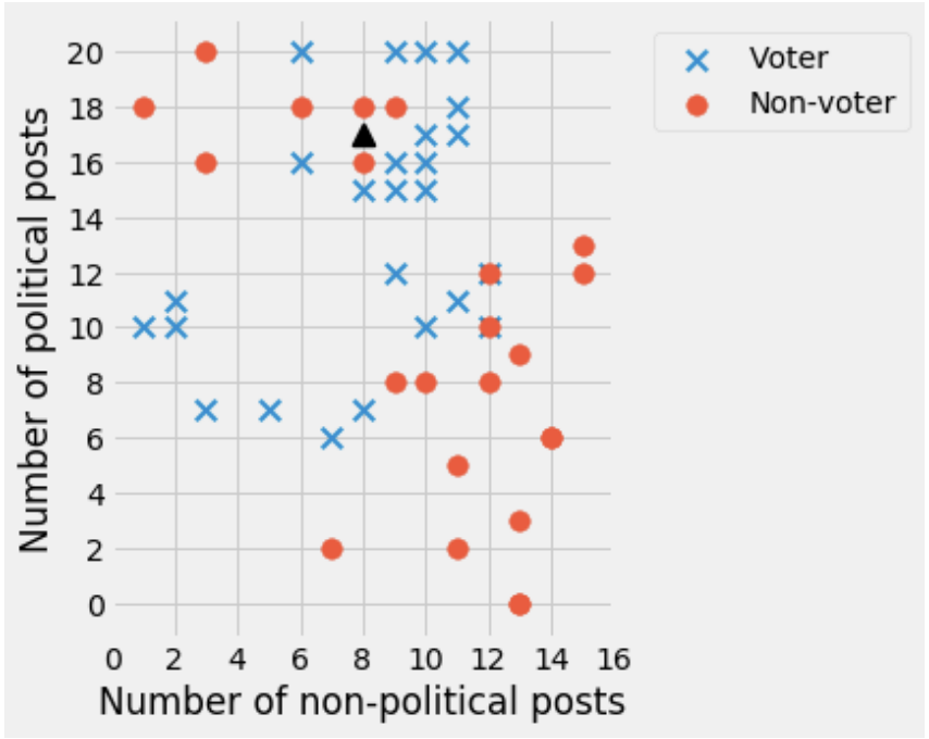
Candidate A decides to train a classifier to predict whether people will vote in the 2020 U.S. election or not. They gather data on voting records from the 2018 U.S. election and decide to use two features: the number of political and non-political posts on social media that the person made in the month leading up to the election. A scatter plot of their initial sample is shown below:
27.4.1 (a)
The candidate is trying to classify the point at (8, 17) shown as a triangle on the graph above. If they use a 3-nearest neighbor classifier, what will their classification be?
- Voter
- Non-voter
Answer
Non-voter. The 3 nearest points to the triangle on the graph are all red circles corresponding to the Non-voter class.27.4.2 (b)
Suppose the candidate randomly divides the data into test and training sets (both much larger than the set shown above), and finds a test set accuracy of 94%. The candidate decides to apply their trained classifier to a test set from another country with lower rates of internet access. Should they expect the accuracy to be the same, higher or lower? Why?
- Same
- Higher
- Lower
Answer
The correct answer is Lower. In regions with lower rates of internet access, people might post less, so they will be in the lower-left corner, and accuracy there is lower due to lack of data.
27.4.3 (c)
Instead of a \(k\)-nearest neighbor classifier, the candidate decides to use a \(d\)-distance classifier. In this classifier, instead of choosing the \(k\) closest neighbors, we’ll instead choose all neighbors within a specified distance \(d\) (including points that are exactly \(d\) units away). If there are an equal number of points with both labels within that distance, choose whichever class you wish.
If \(d = 5\), how would you classify the point at (8, 17) shown as a triangle on the graph above?
- Voter
- Non-voter
Answer
The correct answer is Voter. Within a circular region of radius 5, there are many more points corresponding to the Voter class than Non-voter.27.4.4 (d)
In the above scatter plot, there are 21 points with a label of Voter, and 25 points with a label of Non-voter. On the plot below, draw the approximate decision boundary for a 43-neighbor classifier, or write “Impossible” below if you cannot draw a decision boundary for this classifier. Explain.
Answer
Impossible. A 43-neighbor classifier would always return Non-voter, since there are only 21 points with a label of Voter. No boundary exists.
27.4.5 (e)
When building a \(k\)-nearest-neighbor classifier, increasing \(k\) will always result in which of the below? Select all that apply.
- Higher training accuracy
- Higher test accuracy
- Lower training accuracy
- Lower test accuracy
Answer
While some generalizations can be made about how increasing \(k\) will lead to higher test accuracy, for example, these trends are not always true for all values of \(k\). This is why finding the best value of \(k\) is often part of building our model, and is a hyperparameter that we tune.
27.5 Linear Regression - Sp17 Final Q4 Modified (Extra)
This scatter plot of a sample of 1,000 trips for New York taxis in January 2016 compares distance and cost. The regression line is shown. Two trips of the same length can vary in cost because of waiting times, special fees, taxes, tolls, tips, discounts, etc.
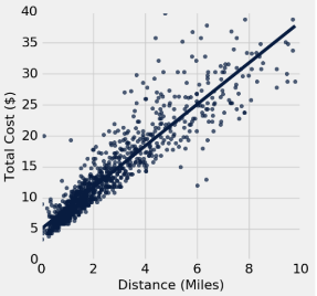
np.average(t.column("Distance")) = 3
np.std(t.column("Distance")) = 2
np.average(t.column("Cost")) = 13
np.std(t.column("Cost")) = 6
correlation(t, "Distance", "Cost") = 0.9
27.5.1 (a)
Convert a trip total cost of $9 to standard units.
Answer
\((9-13)/6 = -2/3\)27.5.2 (b)
What is the slope of the regression line for this sample in dollars per mile?
Answer
\(0.9 * 6 / 2 = 2.7\)27.5.3 (c)
What is the intercept of the regression line for this sample in dollars?
Answer
\(13 - 2.7 * 3 = 4.9\)27.5.4 (d)
If instead we fit a regression line to estimate distance in miles from total cost in dollars, what would be the slope of that line in miles per dollar? Write not enough info if it’s impossible to say.
Answer
\(0.9 * 2 / 6 = 0.3\)27.5.5 (e)
Circle one of (A) True, (B) False, or (C) Not Enough Info to describe the following statement:
The total cost values in this sample are normally distributed.
Answer
False: Most values are between 0 and 2 with a tail to the right.27.5.6 (f)
Circle one of (A) True, (B) False, or (C) Not Enough Info to describe the following statement:
All of the total cost values in this sample are within 3 standard deviations of the mean.
Answer
False: One value is 40, which is larger than 3 * 6 + 13 = 31.27.5.7 (g)
Circle one of (A) True, (B) False, or (C) Not Enough Info to describe the following statement:
At least 88% of the total cost values in this sample are within 3 standard deviations of the mean.
Answer
True: By Chebyshev’s inequality, it must be true. At least \(1-\frac{1}{z^2} = 1 - \frac{1}{9} = 8/9\) or 88.89% are within 3 SDs of the mean for any distribution.27.5.8 (h)
Circle one of (A) True, (B) False, or (C) Not Enough Info to describe the following statement:
The residual costs have a similar average magnitude for short trips (1 mile) and long trips (5+ miles).
Answer
False: There is less variability for shorter rides, and therefore smaller error magnitudes.
27.5.9 (i)
You compute a 95% confidence interval from this sample to estimate the height (fitted value) of the population regression line at 6 miles. Which one of the following could plausibly be the result?
- 5 to 7
- 7 to 19
- 12 to 14
- 15 to 35
- 24 to 26
Answer
The regression estimate for this sample is 25, so that will be the center of the confidence interval. Since it’s a large sample, most resampled estimates will be near to this value. 15 to 35 is not plausible because a resampled regression line would almost never vary so much that it would go through those extreme values.