Contact me by email at ease — I typically respond within a day or so!
22.0.2 Announcements
CautionAnnouncements
The deadline to change grading option for L&S is October 31st.
NoteNote
So far in the course, you have used the bootstrap to estimate multiple different parameters of a population such as the median and mean. You are now capable of building empirical distributions for these sample statistics. An empirical distribution for a sample statistic is usually obtained by repeatedly resampling and calculating the statistic for those resamples (i.e., via bootstrapping!).
Now we will introduce the Central Limit Theorem (CLT), which tells us more about the distribution of the sample mean: if you draw a large random sample with replacement from a population, then, regardless of the distribution of the population, the probability distribution for that sample’s mean is roughly normal, centered at the population mean.
Furthermore, the standard deviation (spread) of the distribution of sample means is governed by a simple equation, shown below:
SD of all possible sample means = \(\frac{\text{Population SD}}{\sqrt{\text{sample size}}}\)
Note, the standard deviation of the sample means is not the standard deviation of the sample. It is the spread of the distribution of all sample means obtain, not of a single sample.
Note that in this question, the empirical distribution of the sample mean is made up from the means of samples drawn from the population (not from resamples from a single sample).
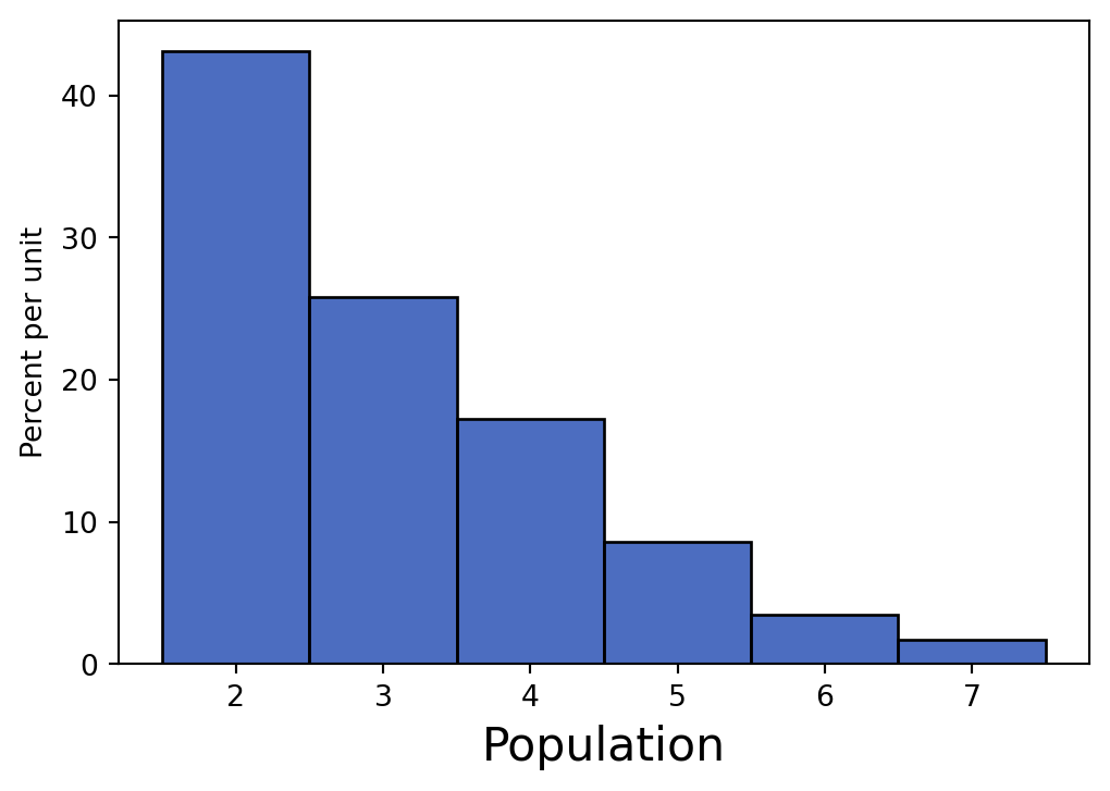
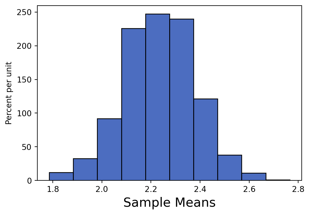
Assume that you have a certain population of interest whose histogram is below.
Cyrus takes many large random samples with replacement from the population with the goal of generating an empirical distribution of the sample mean. What shape do you expect this distribution to have? Which value will it be centered around?
Answer
By the Central Limit Theorem, the distribution will be normal (bell curve), centered around the population mean.
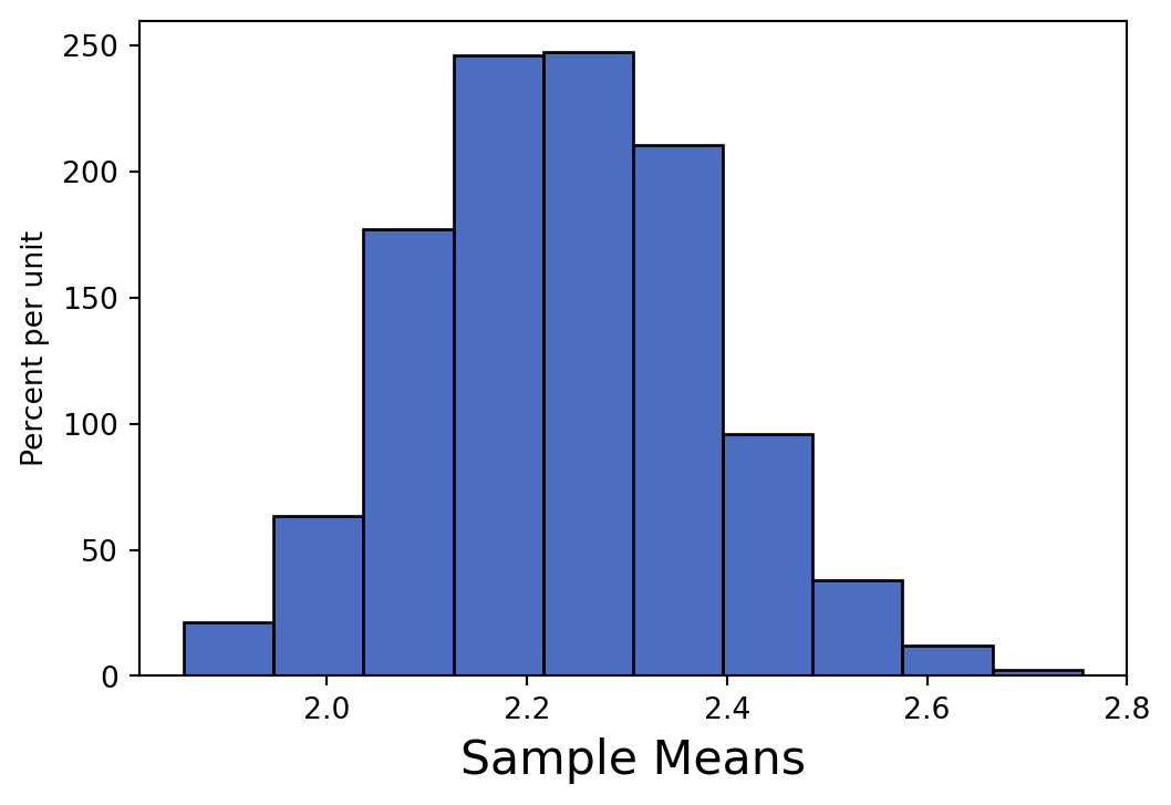
sample_means = make_array()for i in np.arange(1000): sample_means = np.append(sample_means, np.mean(pops.sample().column(0)))Table().with_columns("Sample Means", sample_means).hist("Sample Means")
NoteCentral Limit Theorem: Conditions
There are two key conditions for the Central Limit Theorem (CLT) to apply:
Samples must be large, random, and drawn with replacement (or relatively small compared to the population if sampling without replacement).
The statistic must be a sample sum or sample mean — CLT does not apply to just any statistic.
When solving problems, look for parts of the question that suggest these conditions are met.
22.1.2 (b)
Why are we able to use the CLT to reason about the empirical distribution of the sample mean’s shape if the population data is skewed?
Answer
We are able to use the CLT, as we are drawing large random samples, with replacement, and the statistic is sum or mean. If these conditions are applied, the CLT can be used regardless of the population’s distribution.
Note, given a large enough population, and small relative sample size, we do not have to sample with replacement, as the behavior approaches that of drawing with replacement. This is out of scope for Data 8.
NoteCLT Intuition: Sample Size and Variability
CLT applies regardless of the population’s shape.
Standard deviation of sample means decreases with larger sample sizes:
SD of sample mean = Population SD ÷ √Sample Size
Example: flipping a coin
10 flips → you might see 30% or 70% heads
100 flips → most results will be between 40% and 60% heads
22.1.3 (c)
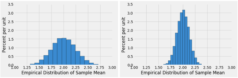
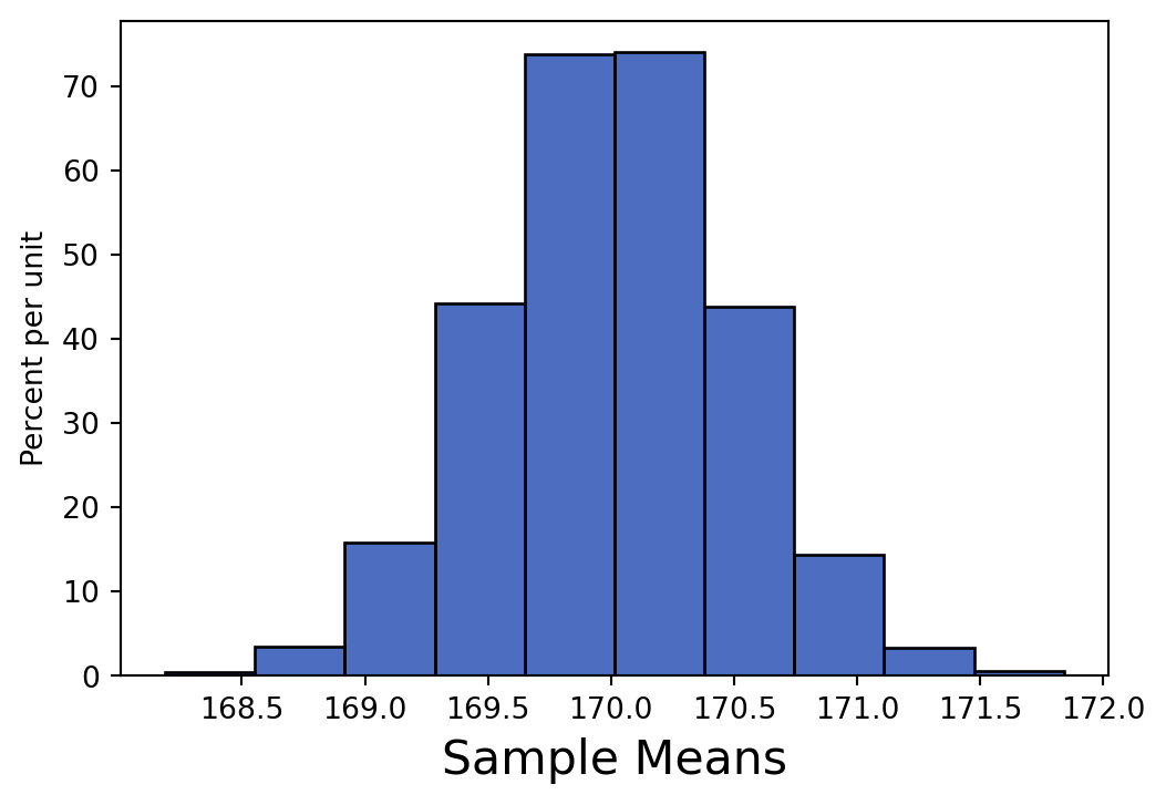
Suppose that Cyrus creates two empirical distributions of sample means, with different sample sizes. Which distribution corresponds to a larger sample size? Why?
Answer
The distribution to the right corresponds to a larger sample size compared to the one to the left. We know based on the spread of the two distributions. The larger the sample size you take, the less variable the distribution of the sample mean becomes.
You can see that increasing the sample size is increasing the denominator in calculating the SD of sample means, which decreases the standard deviation.
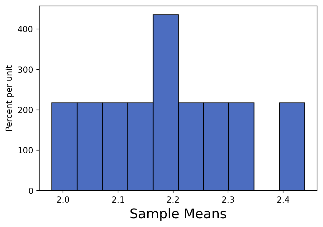
sample_means = make_array()for i in np.arange(10): sample_means = np.append(sample_means, np.mean(pops.sample().column(0)))Table().with_columns("Sample Means", sample_means).hist("Sample Means")
sample_means = make_array()for i in np.arange(1000): sample_means = np.append(sample_means, np.mean(pops.sample().column(0)))Table().with_columns("Sample Means", sample_means).hist("Sample Means")
22.1.4 (d)
Based solely on the information in the histogram, what is an estimate for the standard deviation of the sample mean on the left? How did you determine this?
NoteUnderstanding Points of Inflection
A point of inflection is where a curve transitions from curving upward to curving downward.
No calculus required!
Visual analogy:
Draw a smooth version of your histogram.
Alternatively, imagine placing a downward-facing bowl on top of an upward-facing bowl.
The single point where they touch is the inflection point.
Answer
Approximately 0.3.
This is because the point of inflection on a normal distribution reflects 1 standard deviation away from the mean. Looking at the histogram, we can see that the inflection points occur at around 1.7 and 2.3, with the mean of the histogram being 2.0.
22.1.5 (e)
Suppose you were told that the distribution on the right was generated based on a sample size of 100 and has a standard deviation of 0.2. How big of a sample size would you need if you wanted the standard deviation of the distribution of sample means to be 10 times smaller?
NoteUsing CLT Formulas
Substitute the known values into the SD formula from CLT to find the population SD or compute a new sample size.
This step is mostly arithmetic once you understand the formula.
To divide the SD of the sample means by a factor of 10, we need to multiply the sample size by \(10^2\), which is 100. To skip the calculations, reference the square root law!
UC Berkeley students love studying in Main Stacks! You are working with Lena on constructing a confidence interval for the mean number of hours students spend in Main Stacks each year. To do this, you take a random sample of 400 UC Berkeley students and record how many hours each student spent studying in Main Stacks over the past year. Then, you compute the mean number of hours for your sample; it is 170 hours. You also calculate the standard deviation of your sample to be 10 hours.
22.2.1 (a)
Lena claims that the distribution of all possible sample means is normal with an SD of 0.5 hours. Use this information to construct an approximate 68% confidence interval for the mean hours spent studying in Main Stacks for all UC Berkeley students.
Answer
We know that the distribution is approximately normal and hence we know that roughly 68% of the area under the normal curve (or 68% of the data) is contained within 1 SD of the mean. Therefore, our confidence interval range will be
If the distribution is roughly normal, about 68% of values lie within 1 SD of the mean.
Example: mean = 170 hours, SD = 0.5 hours
CI ≈ [mean ± 1 SD] → [169.5, 170.5]
22.2.2 (b)
If Lena had not told you what the SD of the distribution of sample means was, could you estimate it from the data in the sample? If yes, how? If no, why not?
Answer
We know that the sample size is 400 and that the standard deviation of our sample was 10 hours. Recall the equation for the SD of sample means is
We can substitute the sample SD (10 hours) in place of the population SD in this formula (assuming the sample is representative of the population) and calculate the value!
For large samples, the sample SD is a good approximation of the population SD.
Even if sampling without replacement, the difference is negligible if the sample is very small relative to the population.
This logic is similar to bootstrapping: if the sample represents the population, we can treat the sample SD as the population SD.
22.2.3 (c) (Bonus!)
Suppose Richard and Bing took a different random sample of 400 UC Berkeley students and found a sample mean of 172 hours, with a sample standard deviation of 10 hours. Would it be surprising to observe this sample mean if the true average number of hours all UC Berkeley students spend in Main Stacks is 170?
Answer
If the true population mean is 170 hours and the standard deviation of the sample means is 0.5 (as we saw before), then we can compute how many standard deviations away 172 is from the mean using a z-score: \(z = \frac{172 - 170}{0.5} = 4\). A z-score of 4 is very far in the tails of the normal distribution — much further than what we would expect by random chance. Therefore, yes, it would be surprising to observe a sample mean of 172 hours if the true mean were 170. This might suggest the true population mean is not 170 hours.
true_mean =170true_sd =10n =400repetitions =5000sample_means = []for _ inrange(repetitions): sample = np.random.normal(true_mean, true_sd, n) sample_means.append(np.mean(sample))sim_table = Table().with_column("Sample Means", sample_means)prop_extreme = np.count_nonzero((sim_table.column("Sample Means") >=172) | (sim_table.column("Sample Means") <=168)) / repetitionsprint("Simulated probability of observing 172 or more extreme:", prop_extreme)sim_table.hist("Sample Means")
Simulated probability of observing 172 or more extreme: 0.0
NoteA helpful note.
In Question 1, our large samples drawn with replacement were obtained directly from the population. As a result, our empirical distribution of the sample mean was centered around the population mean.
In contrast, in Question 2, we only have access to a single sample. As a result, we use the sample’s mean and standard deviation in place of the population’s mean and standard deviation, given the assumption that it is a representative sample.
If you bootstrap (resample) from a representative sample and obtain the empirical distribution of the sample means, it will be roughly centered around the original sample’s mean, not the population mean. However, it is helpful to note that as the sample size gets larger, your original sample’s mean will likely get closer and closer to the population mean, by the law of large numbers.
In both situations – whether resampling directly from the population or bootstrapping from a single representative sample – the Central Limit Theorem applies as long as its conditions are met.
22.3 CLT with TLC
You are a super fan of the girl group TLC and are interested in estimating the average amount of plays their songs have online. You generate an 80% confidence interval for this parameter to be [700000, 1200000] based on a random sample of 50 songs using the Central Limit Theorem. Are each of the following statements true or false?
Note: Generally, \(n \geq 30\) is considered the minimum sample size for CLT to take effect!
The value of our population parameter changes depending on our sampling process.
Answer
Our population parameter is fixed. It depends on an entire population that we know to be true. On the other hand, the sample statistic is dependent on what our sample looks like, which can vary. This is what allows us to describe probabilities regarding a confidence interval before we generate them but not after. (see part (d))
22.3.2 (b)
The empirical distribution of any statistic we choose will be roughly normal based on the Central Limit Theorem, but it requires our population to have a normal distribution to begin with.
Answer
The Central Limit Theorem states that the probability distribution of the sum, average, or proportions of a large random sample drawn with replacement will be roughly normal, regardless of the distribution of the population from which the sample is drawn.
22.3.3 (c)
If we generate a 95% confidence interval using the same sample, the interval will be narrower than the original confidence interval because we are more certain of our results.
Answer
Using a 95% confidence level would result in a wider interval than an 80% confidence level. In fact, the 95% confidence interval will envelop the original 80% confidence interval. The “increased confidence” comes from having a wider interval.
arr = make_array()for i in np.arange(1000): arr = np.append(arr, np.mean(tlc_songs.sample().column(0)))print(f'95% Confidence Interval for average plays: [{percentile(2.5, arr)}, {percentile(97.5, arr)}]')print(f'80% Confidence Interval for average plays: [{percentile(10, arr)}, {percentile(90, arr)}]')
95% Confidence Interval for average plays: [890028.7060435255, 973742.332320317]
80% Confidence Interval for average plays: [903280.2501750317, 958748.4629483994]
22.3.4 (d)
Using the same process to generate another 80% confidence interval, there is an 80% chance that the next confidence interval you generate will contain the true average number of plays for TLC songs.
Answer
Before we create the confidence interval, there is an 80% chance that the confidence interval we create next will contain the true population parameter. Confidence refers to the probability associated with our process of generating confidence intervals, not the probability associated with a single well-defined interval.
22.3.5 (e)
There is an 80% chance that a confidence interval we generated contains the true average number of plays for TLC songs.
Answer
Once we have calculated a confidence interval, it is fixed - it either contains the parameter or it does not. There is no chance involved.
NoteConfidence Intervals vs. Confidence Level
When working with confidence intervals (CIs), remember:
Confidence Level refers to the process of creating the interval, not the interval itself after it’s calculated.
Example: flipping a coin
There’s randomness while the coin is in the air.
Once it lands, it’s either Heads or Tails — no randomness remains.
The CI Guide is a helpful resource for understanding these nuances.
22.3.6 (f)
80% of TLC’s songs have between 700,000 and 1,200,000 plays.
Answer
Our confidence interval is estimating the average number of plays but makes absolutely NO claim about what percentage of songs have between 700,000 and 1,200,000 plays. A \(n\)% confidence interval contains \(n\)% of the statistics you simulated, but it does not suggest that \(n\)% of the population is in that interval!
The original sample mean you obtained was approximately 950,000 plays.
Answer
If we sample repeatedly from the original sample to construct the confidence interval, the Central Limit Theorem tells us that the distribution of sample means will be roughly normal and that it will be centered around the sample mean.