6 Discussion 04: More Visualizations, Intro to Functions (from Fall 2025)

6.0.1 Contact Information

Name	Wesley Zheng
Pronouns	He/him/his
Email	wzheng0302@berkeley.edu
Discussion	Wednesdays, 12–2 PM @ Etcheverry 3105
Office Hours	Tuesdays/Thursdays, 2–3 PM @ Warren Hall 101

Contact me by email at ease — I typically respond within a day or so!

6.0.2 Announcements

Announcements

Fill out the Midterm Conflicts Form (QR code in slides).
Complete the Project 1 Partner Matching Form.

Making Sense of Histograms

Histograms help us understand the distribution of one numerical variable. They show how spread out the data is and where it tends to cluster.

Histograms vs. Bar Charts

Histogram: Used for numerical data. You can adjust the bin widths to change how the distribution looks.
Bar Chart: Used for categorical data. Categories are fixed, so there are no adjustable bins.

The X-Axis

The x-axis units match the numerical variable being plotted.
Bins indicate how the range of values is divided up.
Choosing bins that are too narrow or too wide can hide useful information about the distribution.

The Y-Axis

The y-axis is the density scale, showing how “crowded” the data are within each bin.
The area of each bin is proportional to the percent of the data in that bin.
- The total area of the histogram always equals 100% (or 1.0).
- If all the data were in one bin, that bin’s area would represent 100%.
A helpful analogy: a packed Wheeler 150 and a packed Dwinelle 155 both feel crowded, even though the total number of people is different—that’s the idea of density.

6.1 Rents & Ranges

The table below shows the distribution of rents paid by students in Boston. The first column consists of ranges of monthly rent, in dollars. Ranges include the lower bound but not the upper bound. The second column shows the percentage of students who pay rent in each of the ranges.

Code

import numpy as np
from datascience import *
%matplotlib inline

rent = Table().with_columns(
  "Dollars", np.append(np.append(np.append(np.ones(15) * 600, np.ones(25) * 900), np.ones(40) * 1100), np.ones(20) * 1400)
)

Note

Area Principle: The area of a bin is equal to the percentage of data in that bin. The larger the area, the more data lies in that bin.

\[ \text{Area of a bar} = \% \text{ of values in a bin} = \text{width of the bin} \times \text{height of the bin} \]

6.1.1 (a)

Calculate the heights of the bars for the bins listed in the table, with correct units. Recall the Area Principle:

Dollars	Students (%)	Bar Height
500 – 800	15
800 – 1000	25
1000 – 1200	40
1200 – 1600	20

Answer

Dollars	Students (%)	Bar Height
500 – 800	15	0.050%
800 – 1000	25	0.125%
1000 – 1200	40	0.200%
1200 – 1600	20	0.050%

Calculation (demonstrated on the 500-800 bin): $\frac{area}{width} = \frac{15\%}{\$800 - \$500} = 0.050\%$ per dollar

6.1.2 (b)

Draw a histogram of the data. Make sure you label your axes!

Height vs. Area

A larger area does not always mean a taller bar.

The area depends on both the width and the height of the bin.
A wide bin might have a large area but still a relatively short height.

This is why you should always connect the shape of the histogram back to the area principle.

Answer

Code

rent.hist("Dollars", bins = [500, 800, 1000, 1200, 1600])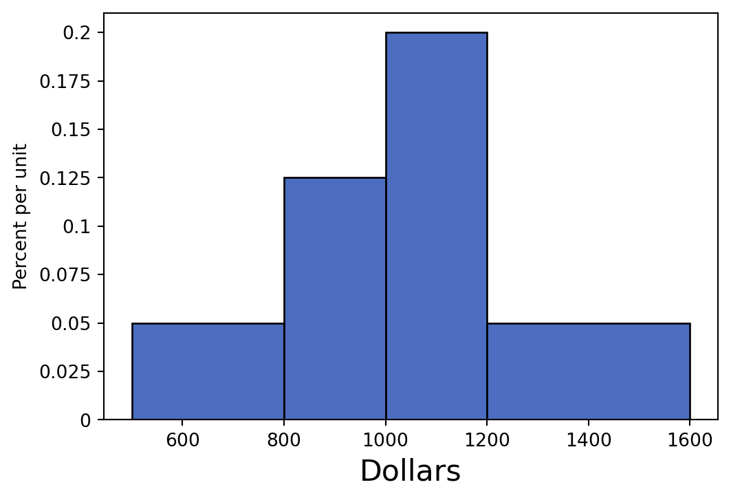

6.1.3 (c)

True or False: If we combine the [500, 800) and [800, 1000) bins together, the height of the new bin would be greater than the heights of both of the old bins. Please explain your answer.

Answer

False: When we combine bins together, the height of the new bin is the weighted average of the old bin heights. Thus, the new bin height will be greater than the [500, 800) bin, but less than the [800, 1000) bin. If we calculate the new height, it will be:

$\text{new height}$ = $\frac{area}{width} = \frac{40\%}{(\$800 - \$500) + (\$1000 - \$800)} = 0.08\%$ per dollar

Combining Bins

When two bins are combined, the new height is like an average.

The height of the combined bin will never exceed the tallest of the original bins.
This is just like averages in general—an average can never be larger than the maximum value.

Code

rent.hist("Dollars", bins = [500, 1000, 1200, 1600])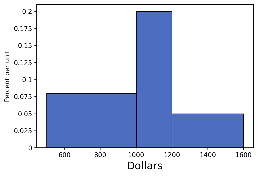

6.2 Fun(ctions)

Code

import warnings
warnings.filterwarnings("ignore")
import random

6.2.1 (a)

After learning about them in Data 8, Tim wants to write a function that can calculate the hypotenuse of any right triangle. He wants to use his function to assign C to the hypotenuse of a right triangle with legs (sides adjacent to the hypotenuse) A and B. However, he’s made many mistakes. Which ones can you identify?

Hint: There are 5 unique issues. Assume that numpy has been imported as np.

Code

A = 3
B = 4

def hypotenuse(a, b)
  squares = make_array(side1, side2) * 2
  sum = sum(squares)
  squareroot = np.sqrt(sum)
  print(squareroot)
C = hypotenuse(A, B) # C should be the numerical result

Answer

Issue 1: the function is missing a colon : after the arguments list.

def hypotenuse(a, b)
  squares = make_array(side1, side2) * 2
  sum = sum(squares)
  squareroot = np.sqrt(sum)
  print(squareroot)
C = hypotenuse(A, B) # C should be the numerical result

  Cell In[6], line 1
    def hypotenuse(a, b)
                        ^
SyntaxError: expected ':'

Issue 2: squares should be squared with ** not *

Issue 3: We need to be consistent with our argument names so they get accurately assigned throughout the function. We can either replace a and b with side1 and side2, or vice versa.

def hypotenuse(a, b):
  squares = make_array(side1, side2) * 2
  sum = sum(squares)
  squareroot = np.sqrt(sum)
  print(squareroot)
C = hypotenuse(A, B) # C should be the numerical result

---------------------------------------------------------------------------
NameError                                 Traceback (most recent call last)
Cell In[7], line 6
      4   squareroot = np.sqrt(sum)
      5   print(squareroot)
----> 6 C = hypotenuse(A, B) # C should be the numerical result

Cell In[7], line 2, in hypotenuse(a, b)
      1 def hypotenuse(a, b):
----> 2   squares = make_array(side1, side2) * 2
      3   sum = sum(squares)
      4   squareroot = np.sqrt(sum)

NameError: name 'side1' is not defined

Issue 4: The function will print the value of squareroot but will not return it, which means we will not have access to the value of squareroot anymore. That is, we will not be able to assign it to any values or use it as the argument to any functions! In this case, C will not be equal to anything (it will actually be None)!

Return vs. Print

It’s important to understand the difference between return and print.

print just displays something on the screen—it doesn’t give you back a usable value. In fact, it returns None.
return gives back a value you can save in a variable and use later.

If you want to keep and work with the result of a function, you should use return.

Function Arguments and Scope

Inside a function:
* Argument names are placeholders—they can be named anything, but they must be used consistently within the function.
* Variables defined inside the function exist only inside the function. They disappear once the function finishes running.

This is called scope.

Issue 5: When we assign sum to a number we have lost the original behavior of the built-in sum function. We should not re-assign variable names. (Note: in this specific question the redefined sum is a local variable and is only scoped within the hypotenuse function, though this is out of scope of Data 8. You should generally never override any function name, regardless of the scope of the variable.)

Naming Variables Safely

Avoid using protected names like sum or max.

These are built-in Python functions. If you reuse them as variable names, you may cause errors in your code and with the autograder.
You can still use short or non-descriptive names if needed—just avoid overwriting protected ones.

def hypotenuse(a, b):
  squares = make_array(a, b) * 2
  sum = sum(squares)
  squareroot = np.sqrt(sum)
  print(squareroot)
C = hypotenuse(A, B) # C should be the numerical result

---------------------------------------------------------------------------
UnboundLocalError                         Traceback (most recent call last)
Cell In[8], line 6
      4   squareroot = np.sqrt(sum)
      5   print(squareroot)
----> 6 C = hypotenuse(A, B) # C should be the numerical result

Cell In[8], line 3, in hypotenuse(a, b)
      1 def hypotenuse(a, b):
      2   squares = make_array(a, b) * 2
----> 3   sum = sum(squares)
      4   squareroot = np.sqrt(sum)
      5   print(squareroot)

UnboundLocalError: cannot access local variable 'sum' where it is not associated with a value

def hypotenuse(a, b):
  squares = make_array(a, b) * 2
  sum_of_squares = sum(squares)
  squareroot = np.sqrt(sum_of_squares)
  print(squareroot)
C = hypotenuse(A, B) # C should be the numerical result
print(C) # C is actually None now!

3.74165738677
None

Fully correct implementation of the function should be:

def hypotenuse(a, b):
  squares = make_array(a, b) * 2
  sum_of_squares = sum(squares)
  squareroot = np.sqrt(sum_of_squares)
  return squareroot
C = hypotenuse(A, B) # C should be the numerical result
C

3.7416573867739413

6.2.2 (b)

Write a function that takes in the following arguments:

tbl: a table.
col: a string, name of a column in tbl.
n: an int.

The function should return a table that contains the rows that have the $n$ largest values for the specified column.

def top_n(tbl, col, n):
  sorted_tbl = __________________________________________________
  top_n_rows = __________________________________________________
  return ________________________________________________________

Answer

def top_n(tbl, col, n):
    sorted_tbl = tbl.sort(col, descending = True)
    top_n_rows = sorted_tbl.take(np.arange(n))
    return top_n_rows

table = Table().with_columns(
  "Some Column", [10, 1, 100, 10000, 1000]
)

table

Some Column
10
1
100
10000
1000

top_n(table, "Some Column", 3)

Some Column
10000
1000
100

6.3 Sheng Kee Fridays

Dagny’s favorite activity to celebrate Fridays is buying pastries at Sheng Kee before class. She stores her purchase data in a table, pastries, to keep track of her spending. Assume she never purchases the same item twice. Each row represents an individual purchase. The first few rows look like this:

Code

pastries = Table().with_columns(
    'item', ['Hot Dog Bun', 'Yudane Milk Bun', 'Summer Romance', 'Pineapple Bun', 'Ham and Cheese Croissant'],
    'category', ['Savory', 'Sweet', 'Sweet', 'Sweet', 'Savory'],
    'price', [2.75, 2.99, 2.79, 2.45, 3.15],
    'satisfaction', [8.5, 9.0, 10.0, 7.75, 7.25]
)

pastries

item	category	price	satisfaction
Hot Dog Bun	Savory	2.75	8.5
Yudane Milk Bun	Sweet	2.99	9
Summer Romance	Sweet	2.79	10
Pineapple Bun	Sweet	2.45	7.75
Ham and Cheese Croissant	Savory	3.15	7.25

The table has 4 columns:

item (string): name of the pastry.
category (string): whether the pastry is sweet or savory.
price (float): price of the pastry.
satisfaction (float): how satisfied (out of 10) Dagny was after eating the pastry.

Practicing with Tables

Working with tables involves a wide set of operations:

.column(), .with_columns(), .where(), .sort(), .group(), .apply()
Selecting rows with tbl.take()
Using NumPy functions like np.mean() and np.arange()

These tools let us create new columns, operate on them, and select multiple rows at once. Practicing these now will make exam-style questions much easier.

6.3.1 (a)

Write a line of code to calculate the average satisfaction Dagny felt after eating sweet pastries.

_________(pastries._______(__________________).column(________))

Answer

np.mean(pastries.where('category', are.equal_to('Sweet')).column('satisfaction'))

8.9166666666666661

6.3.2 (b)

Dagny is curious if the average price for savory pastries is higher than the average price for sweet pastries. Write a line of code that will output the category that is more expensive.

pastries.__________________(____________________, ____________________)
        .sort(___________________________, ___________________________)
        .column(_________________________________________).item(______)

Answer

pastries.group("category", np.mean).sort("price mean", descending=True).column("category").item(0)

'Savory'

Note the new column name after .group is price mean. The .sort must take in the correct column name. Alternatively you may use the index of the column after grouping.

6.3.3 (c)

Dagny’s budget is getting tight, and she wants to buy pastries that will give her the most satisfaction per dollar. Write lines of code that will help us achieve this.

6.3.3.1 (i)

First, create an array that contains each purchase’s satisfaction per dollar. Then, add a new column called “satisfaction per $”, to the pastries table.

score_array = pastries._______(_________) / pastries._______(_________)
pastries = ______.with_column(_____________, __________________)

Answer

score_array = pastries.column('satisfaction') / pastries.column('price')
pastries = pastries.with_column('satisfaction per $', score_array)

pastries

item	category	price	satisfaction	satisfaction per $
Hot Dog Bun	Savory	2.75	8.5	3.09091
Yudane Milk Bun	Sweet	2.99	9	3.01003
Summer Romance	Sweet	2.79	10	3.58423
Pineapple Bun	Sweet	2.45	7.75	3.16327
Ham and Cheese Croissant	Savory	3.15	7.25	2.30159

6.3.3.2 (ii)

Dagny defines a function score that takes in satisfaction and price (in that order) and returns the satisfaction per dollar. Find a different way to compute score_array.

score_array = pastries._________________(__________________, __________________, __________________)

Code

def score(satisfaction, price):
    return satisfaction / price

Answer

score_array = pastries.apply(score, "satisfaction", "price")

score_array

array([ 3.09090909,  3.01003344,  3.58422939,  3.16326531,  2.3015873 ])

6.3.3.3 (iii)

Dagny is interested in finding the pastries in the table with the top 3 satisfaction values per dollar. Write code that will output the names of these items as an array.

pastries_sorted = pastries.__________(__________, __________)
pastries_sorted.__________(__________).column(__________)

Answer

pastries_sorted = pastries.sort('satisfaction per $', descending = True)
pastries_sorted.take(np.arange(3)).column('item')

array(['Summer Romance', 'Pineapple Bun', 'Hot Dog Bun'],
      dtype='<U24')

6.3.4 (d) (Bonus!)

Write a line of code to calculate the total amount Samiksha spent on pastries. Assume all of her pastry purchases are recorded in the table.

Answer

sum(pastries.column('price'))

14.130000000000001

6.4 Insurance (Optional)

The table insurance contains one row for each beneficiary that is covered by a particular insurance company:

Code

insurance = Table.read_table("insurance.csv")
insurance.show(3)

age	bmi	smoker	region	cost
25	20.8	no	southwest	3208.79
25	30.2	yes	southwest	33900.7
62	32.1	no	northeast	1355.5

... (20198 rows omitted)

The table contains five columns:

age (int): the age of the beneficiary.
bmi (float): the Body Mass Index (BMI) of the beneficiary.
smoker (string): indicates whether the beneficiary smokes.
region (string): the region of the United States where the beneficiary lives.
cost (float): the total amount in medical costs that the insurance company paid for this beneficiary last year.

(Fall 2018 Midterm Question 2 Modified)

In each part below, fill in the blanks to achieve the desired outputs.

6.4.1 (a)

A scatter plot comparing the amount paid last year vs. BMI (titles are usually written as Y vs. X) for only the beneficiaries whose costs exceeded $25,000. Each dot on the scatter plot should represent one beneficiary.

high_cost = _________.______(_______, _______________________)
_____.___________(__________________, _________________)

Answer

high_cost = insurance.where("cost", are.above(25000))
high_cost.scatter("bmi", "cost")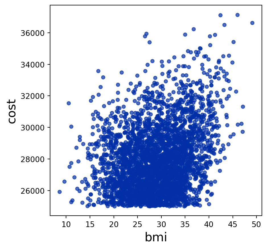

6.4.2 (b)

Write a function that takes an age as an argument, and returns the average BMI among all beneficiaries of that age.

Functions in Tables

Functions are a critical part of working with tables.

You will use them heavily in Project 1.
A function lets you define a reusable operation that can then be applied to entire columns.

def average_bmi(age):
  right_age = insurance.where(________________, ________________)
  bmis = right_age._______________(______________)
  avg = sum(bmis) / len(bmis)
  _____________________________________

Answer

def average_bmi(age):
    right_age = insurance.where("age", age)
    bmis = right_age.column("bmi")
    avg = sum(bmis) / len(bmis)
    return avg

average_bmi(30)

28.487799043062214