9 CS 189 Discussion 09: Backpropagation & CNNs (From Spring 2026)
9.0.1 Contact Information
| Name | Wesley Zheng |
| Pronouns | He/him/his |
| wzheng0302@berkeley.edu | |
| Discussion | Wednesdays, 11–12 PM @ Wheeler 120 & Wednesdays, 3-4 PM @ Hildebrand Hall B51 |
| Office Hours | Tuesdays, 11–1 PM @ Cory Courtyard |
9.1 Backprop in Practice: Staged Computation (F25 Dis8 Q1)
We will apply backpropagation for the function \(f(x,y,z) = (x+y)z\).
Core Idea
- Efficiently computes gradients of loss w.r.t. all parameters
- Uses chain rule + reuses computations
Forward Pass
- Compute activations layer-by-layer
- Store intermediate values
- Produce prediction → compute loss
Backward Pass
- Propagate error output → input
- Apply chain rule: \[ \frac{dL}{dw} = \frac{dL}{da}\frac{da}{dw} \]
- Reuse gradients (dynamic programming style)
Local Gradients
- Each layer computes its own derivative
- Modular across layers
Requirements
- Operations must be differentiable (or use subgradients)
9.1.1 (a)
Decompose \(f\) into two simpler functions.
Answer
We can conveniently express \(f\) as: \(g=x+y\), \(f=gz\). The original \(f(x,y,z)\) expression is simple enough to differentiate directly, but this particular approach of thinking about it in terms of its decomposition can help with understanding the intuition behind backprop.9.1.2 (b)
Draw the computation graph that represents \(f\) following the composition from part (a).
Answer
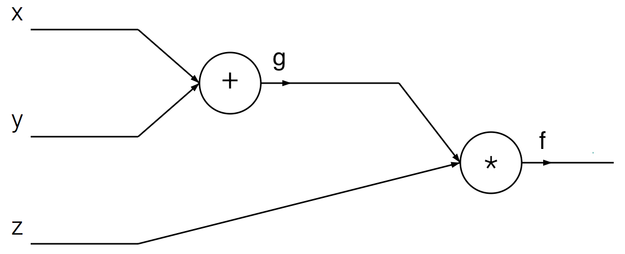
9.1.3 (c)
Write the steps of the forward pass and backward pass through the network.
Answer
\[\begin{array}{l} \textbf{Forward pass:} g = x + y, \\[2pt] f = g \cdot z. \\[10pt] \textbf{Backward pass:} \\[4pt] \text{Backprop through } f = g z: \\[2pt] \dfrac{\partial f}{\partial z} = g, \quad \dfrac{\partial f}{\partial g} = z. \\[8pt] \text{Backprop through } g = x + y \text{ (using the chain rule):} \\[2pt] \dfrac{\partial f}{\partial x} = \dfrac{\partial g}{\partial x} \cdot \dfrac{\partial f}{\partial g} = 1 \cdot \dfrac{\partial f}{\partial g} = \dfrac{\partial f}{\partial g}, \\[6pt] \dfrac{\partial f}{\partial y} = \dfrac{\partial g}{\partial y} \cdot \dfrac{\partial f}{\partial g} = 1 \cdot \dfrac{\partial f}{\partial g} = \dfrac{\partial f}{\partial g}. \end{array}\]
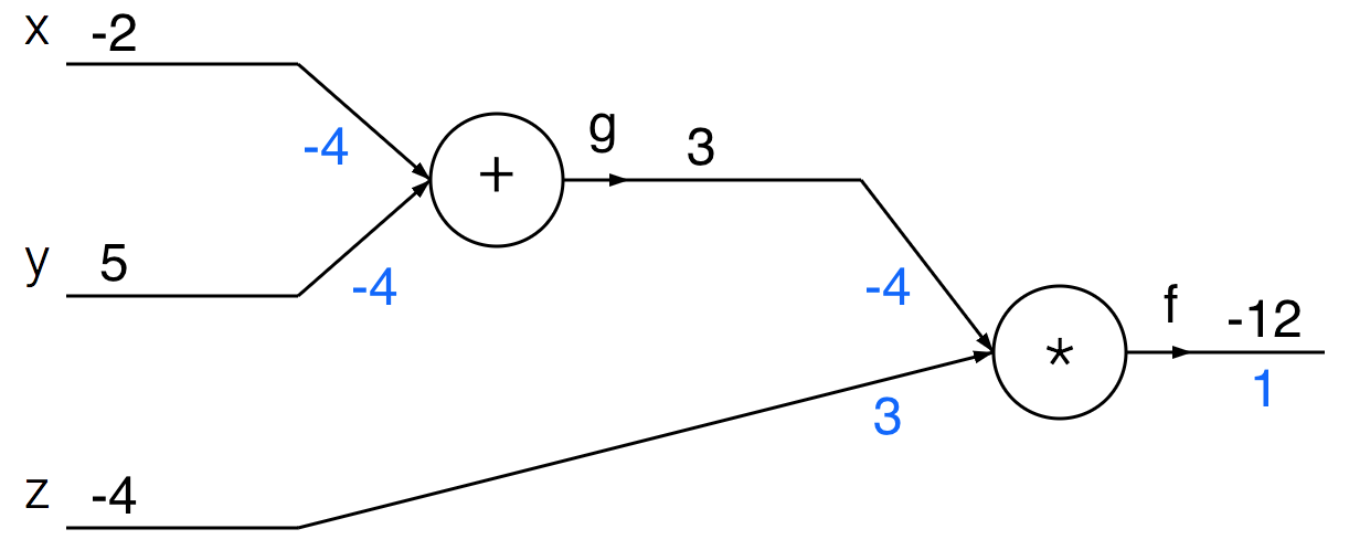
9.1.4 (d)
Update your network drawing with the intermediate values in the forward and backward pass using the inputs \(x = -2\), \(y = 5\), and \(z = -4\).
Answer
We first run the forward pass (shown in black) of the network, which computes values from inputs to output. Then, we do the backward pass (blue), which starts at the end of the network and recursively applies the chain rule to compute the gradients.
9.2 Convolution Operation in CNNs (F25 Dis9 Q1)
In this question, we will look at the mechanism of weight sharing in convolutions. Suppose that we have an input vector with \(D=9\) dimensions: \[\mathbf{x} = [\,x_1 \quad x_2 \quad ... \quad x_9\,]^T.\]
We compute a 1D convolution with the kernel filter that has \(K=3\) weights (parameters): \[\mathbf{k} = [\,k_1 \quad k_2 \quad k_3\,]^T.\]
Core Idea
- Learn spatial features from grid-like data (e.g., images)
- Exploit local structure + parameter sharing
Convolution Layer
- Apply small filters (kernels) across input
- Same weights reused across locations
Feature Maps
- Each map highlights a specific feature
Activation (e.g., ReLU)
- Adds non-linearity
Pooling (Downsampling)
- Reduces spatial size (e.g., max pooling)
- Keeps important features, reduces computation
Hierarchy of Features
- Early layers → edges
- Middle layers → textures/parts
- Deep layers → objects
Fully Connected Layers
- Combine extracted features for final prediction
- Used near output
Outcome
- Strong performance on vision tasks (classification, detection, etc.)
9.2.1 (a)
What’s the output dimension if we apply filter \(\mathbf{k}\) with no padding and stride of 1? What’s the first element of the output? What’s the last element?
Answer
The output dimension is 9 - 3 + 1 = 7.
Each output is one dot product of \(\mathbf{k}\) with a length-\(3\) window of \(\mathbf{x}\); stride \(1\) slides the window one index at a time, giving \(D-K+1\) outputs.
The first element is \(k_1x_1 + k_2x_2 + k_3x_3\) and the last element is \(k_1x_7 + k_2x_8 + k_3x_9\).
First window lines up with \((x_1,x_2,x_3)\); last window lines up with \((x_7,x_8,x_9)\) so the final kernel weight still multiplies \(x_9\).
9.2.2 (b)
What’s the output dimension if we apply filter \(\mathbf{k}\) with padding of size 1 and stride of 2? What’s the first element of the output? What’s the second element?
Answer
For the second example, the output dimension would be \((9+2-3)//2 + 1 = 5\).
Padding \(p=1\) adds one entry on each side (zeros here), so effective length is \(9+2\); stride \(2\) counts every other alignment; // is floor division after the fraction.
The first element is \(k_10 + k_2x_1 + k_3x_2\) and the second element would be \(k_1x_2 + k_2x_3 + k_3x_4\).
Here \(k_10\) denotes \(k_1\) multiplying the left padded zero; the first window is \((0,x_1,x_2)\). Stride \(2\) shifts the window so the next triple is \((x_2,x_3,x_4)\).
9.2.3 (c)
Recall that CNN filters have the property of weight sharing, meaning that different portions of an image can share the same weight to extract the same set of features. A convolution is actually a linear operation, which we can express as \(\mathbf{x}' = \mathbf{K}\mathbf{x}\) for some weight matrix \(\mathbf{K}\). Find \(\mathbf{K}\) for the convolution applied in part (a). What is its dimension?
Answer
The input size is \(D=9\) and the output size shrinks by \(K-1=2\), so \(\mathbf{K}\) has a dimension of \(\mathbb{R}^{7\times9}\) and is given by \[ \mathbf{K} = \begin{bmatrix} k_1 & k_2 & k_3 & 0 & 0 & \cdots & 0\\ 0 & k_1 & k_2 & k_3 & 0 & \cdots & 0\\ & & & \vdots & & & \\ 0 & \cdots & 0 & k_1 & k_2 & k_3 & 0\\ 0 & \cdots & 0 & 0 & k_1 & k_2 & k_3 \end{bmatrix}.\]
Seven rows for seven outputs; each row encodes one sliding window as a dot product with \(\mathbf{x}\). The repeated shifted triple \((k_1,k_2,k_3)\) is exactly weight sharing written as a sparse banded matrix.
9.2.4 (d)
Consider now a 2-dimensional example with the following kernel filter and image: \[\mathbf{K} = \frac{1}{4} \begin{bmatrix} 1 & 1\\ 1 & 1 \end{bmatrix} \hspace{10mm} \mathbf{X} = \begin{bmatrix} 1 & 2 & 3\\ 4 & 5 & 6\\ 7 & 8 & 9 \end{bmatrix} \]
Using no padding and a stride of 1, compute the output, and describe the effect of this filter.
Answer
The output is \[ \begin{bmatrix} 3 & 4 \\ 6 & 7 \end{bmatrix}. \]
Each entry is an average of a \(2\times 2\) block of \(\mathbf{X}\) (e.g. top-left uses \(1,2,4,5\)), consistent with the all-ones kernel scaled by \(\frac{1}{4}\).
9.2.5 (e)
We want to know the general formula for computing the output dimension of a convolution operation. Suppose we have a square input image of dimension \(W \times W\) and a \(K \times K\) kernel filter. If we assume stride of 1 and no padding, what’s the output dimension \(W'\)? What if we applied stride of \(s\) and padding of size \(p\), how would the dimension change?
Answer
With a stride length of one and no padding, the output dimension will be \(W' = W - K + 1\).
With a stride of \(s\) and padding of size \(p\), the output dimension will be \(\lfloor\frac{W + 2p - K}{s}\rfloor + 1\). We include a \(+2p\) because the padding is equivalent to adding extra terms on both the left and right side of the array. Dividing by \(s\) follows from the fact that we increment our counter by \(+s\) instead of \(+1\) when sliding along the image. The floor division operator ensures that the resulting output is an integer.
\(W+2p\) is the padded side length; subtract \(K\) for the first valid window span; divide by \(s\) counts how many stride steps fit; \(+1\) counts the initial placement; floor drops a partial tail if the last stride would overshoot.