11 CS 189 Discussion 11: Transformers II (From Spring 2026)
11.0.1 Contact Information
| Name | Wesley Zheng |
| Pronouns | He/him/his |
| wzheng0302@berkeley.edu | |
| Discussion | Wednesdays, 11–12 PM @ Wheeler 120 & Wednesdays, 3-4 PM @ Hildebrand Hall B51 |
| Office Hours | Tuesdays, 11–1 PM @ Cory Courtyard |
11.1 Positional Encoding (F25 Dis11 Q1)
Core Idea
- Self-attention is permutation-invariant → no inherent notion of order
- Positional encoding injects sequence order into token representations
Types of Positional Encoding
- Absolute encoding
- Encodes position index directly
- Each token gets a position-specific embedding
- Encodes position index directly
- Relative encoding
- Encodes distance between tokens
- Shift-invariant → generalizes across sequence lengths
- Encodes distance between tokens
Rotary Positional Embeddings (RoPE)
- Rotate embeddings by position-dependent angle
- Encodes position through geometric transformation
- Attention scores depend only on relative positions
11.1.1 (a)
Why do we need positional encoding? Describe a situation where word-order information is necessary for the task performed.
Answer
Positional encoding is needed because the self-attention mechanism is permutation-invariant over its inputs (i.e., it treats all positions symmetrically). Without additional information, the model cannot tell whether a token appeared at the beginning, middle, or end of the sequence, nor can it distinguish different word orders.
If you permute the rows of \(X\), self-attention outputs permute the same way—order is not in the architecture until you inject it (additive/sinusoidal/RoPE/etc.).
11.1.2 (b)
What is relative positional encoding? How is it different from absolute positional encoding?
Answer
In absolute positional encoding, each position \(n\) in a sequence of length \(N\) has its own encoding \(r_n\). The input token embedding \(x_n\) is combined (e.g., by addition) with \(r_n\) so that the final input depends on the absolute index of each token.
Think “token \(n\) carries a label \(n\)”: the representation explicitly knows whether it is token 0 vs token 100, even before attending.
In relative positional encoding, what matters is not the absolute index of each token but the distance between the query position and the key position it is attending to. The encoding used when a query at position \(n\) attends to a key at position \(i\) depends only on \((n-i)\), not on \(n\) or \(i\) individually. This makes the attention mechanism naturally shift-invariant and better able to generalize across sequence lengths.
Think “only offsets matter”: sliding the whole window left/right should not change pairwise interactions if relative distances stay the same—useful when train/test sequence lengths differ.
11.1.3 (c)
Rotary positional embeddings (RoPE) are a way of encoding token positions by rotating pairs of embedding dimensions by an angle that grows with the position index, so that inner products between tokens automatically depend only on their relative positions. They’ve become a de-facto default in many modern LLMs.
Consider a sequence of \(N\) two-dimensional vectors \[ x_n := \bigl( x_n^{(1)}, x_n^{(2)} \bigr), \quad n = 1,2,\dots, N. \] For a parameter \(\theta \in \mathbb{R}\), the RoPE encoding at position \(n\) is \[ \operatorname{RoPE}(x_n,n) = R(n\theta) x_n, \qquad \text{where} \qquad R(\alpha) := \begin{pmatrix} \cos\alpha & -\sin\alpha \\ \sin\alpha & \cos\alpha \end{pmatrix}. \] Show that the dot product between two RoPE-encoded vectors depends only on their relative positions. In particular, prove that for any integers \(m\), \(n\), and \(k\), the following holds: \[ \operatorname{RoPE}(x,m)^\top \operatorname{RoPE}(y,n) \;=\; \operatorname{RoPE}(x,m+k)^\top \operatorname{RoPE}(y,n+k). \]
Answer
We have \[ \operatorname{RoPE}(x,m) = R(m\theta)x, \qquad \operatorname{RoPE}(y,n) = R(n\theta)y. \]
Consider their dot product: \[ \begin{align*} \operatorname{RoPE}(x,m)^\top \operatorname{RoPE}(y,n) &= (R(m\theta)x)^\top (R(n\theta)y) \\ &= x^\top R(m\theta)^\top R(n\theta) y. \end{align*} \]
Pull transposes onto rotations: \((AB)^\top = B^\top A^\top\), so the middle becomes \(R(m\theta)^\top R(n\theta)\).
The matrix \(R(\alpha)\) is a \(2\times 2\) rotation matrix, so the following properties hold: \[ R(\alpha)^\top = R(-\alpha), \quad R(\alpha) R(\beta) = R(\alpha + \beta). \]
Rotations form a group: transpose = inverse rotation (\(R(\alpha)^\top=R(-\alpha)\)), and composing rotations adds angles.
Therefore, \[ R(m\theta)^\top R(n\theta) = R(-m\theta)R(n\theta) = R\bigl((n-m)\theta\bigr). \]
The two angles \(-m\theta\) and \(n\theta\) combine to \((n-m)\theta\): the score machinery only “sees” the offset between query and key positions.
Using this expression in the dot product we computed earlier, we see
\[ \operatorname{RoPE}(x,m)^\top \operatorname{RoPE}(y,n) = x^\top R\bigl((n-m)\theta\bigr) y, \] which depends only on the difference \((n-m)\), i.e., on the positions of \(x\) and \(y\).
Now consider shifting both positions by an integer \(k\): \[ \operatorname{RoPE}(x,m+k)^\top \operatorname{RoPE}(y,n+k) = x^\top R\left(\bigl((n+k)-(m+k)\bigr)\theta\right)\,y = x^\top R\bigl((n-m)\theta\bigr) y. \]
Shifting both indices by \(k\) cancels inside \((n+k)-(m+k)=n-m\): global index moves, relative offset stays.
This equals the previous expression, so \[ \operatorname{RoPE}(x,m)^\top \operatorname{RoPE}(y,n) = \operatorname{RoPE}(x,m+k)^\top \operatorname{RoPE}(y,n+k). \]
This now shows that the RoPE-encoded dot product is invariant to a global shift of both token positions and depends only on their positions relative to one another.11.2 Matching Similarity Matrices to Attention Heatmaps (F25 Dis11 Q2)
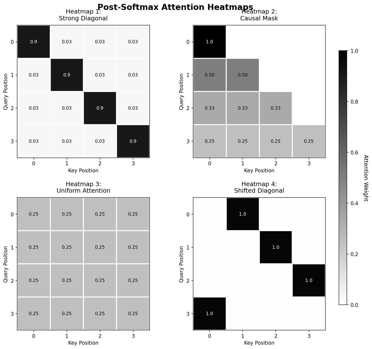
Recall that in self-attention mechanisms, we compute the key-query similarity matrix \(QK^T\), scale the matrix by \(\frac{1}{\sqrt{D_k}}\), and then apply the softmax function row-wise to obtain attention scores. Understanding how pre-softmax similarity scores translate to post-softmax attention weights is crucial for interpreting attention patterns. Below are four \(4 \times 4\) pre-softmax similarity matrices and four corresponding post-softmax attention heatmaps. Your task is to match each pre-softmax matrix to its corresponding heatmap and explain the transformation.
Pre-softmax matrices:
Matrix A: \[ \begin{bmatrix} 2 & 2 & 2 & 2 \\ 2 & 2 & 2 & 2 \\ 2 & 2 & 2 & 2 \\ 2 & 2 & 2 & 2 \end{bmatrix} \]
Matrix B: \[ \begin{bmatrix} 10 & 1 & 1 & 1 \\ 1 & 10 & 1 & 1 \\ 1 & 1 & 10 & 1 \\ 1 & 1 & 1 & 10 \end{bmatrix} \]
Matrix C: \[ \begin{bmatrix} 5 & -\infty & -\infty & -\infty \\ 5 & 5 & -\infty & -\infty \\ 5 & 5 & 5 & -\infty \\ 5 & 5 & 5 & 5 \end{bmatrix} \]
Matrix D: \[ \begin{bmatrix} -\infty & 5 & -\infty & -\infty \\ -\infty & -\infty & 5 & -\infty \\ -\infty & -\infty & -\infty & 5 \\ 5 & -\infty & -\infty & -\infty \end{bmatrix} \]
Post-softmax heat maps (darker = higher attention weight):
11.2.1 (a)
Match each pre-softmax matrix (A-D) to its corresponding heatmap (1-4). Provide brief reasoning for each match.
Answer
- Matrix A → Heatmap 3: All values are identical (2), so after applying softmax to each row, each token pair gets equal attention weight: \(\frac{e^2}{4e^2} = \frac{1}{4} = 0.25\).
Uniform logits \(\Rightarrow\) uniform softmax: every column in a row gets the same mass (here \(0.25\) for length-4).
- Matrix B → Heatmap 1: The diagonal has much larger values (10) than off-diagonal (1). After softmax: diagonal gets \(\frac{e^{10}}{e^{10} + 3e^1} \approx 0.9997\), off-diagonal gets \(\frac{e^1}{e^{10} + 3e^1} \approx 0.0001\).
Large logit gaps explode under exp—softmax becomes nearly one-hot on the max entry (strong self-attention / “look at myself”).
- Matrix C → Heatmap 2: This is a causal mask with \(-\infty\) in the upper triangle. After applying softmax, \(e^{-\infty} = 0\), so the upper triangle becomes 0. The lower triangle has uniform values, so attention is distributed equally among valid positions.
\(-\infty\) logits zero out forbidden positions; remaining logits tie \(\Rightarrow\) uniform over allowed past tokens (causal attention often looks flat before content is added).
- Matrix D → Heatmap 4: The positions \((0,1), (1,2), (2,3), (3,0)\) have value 5, while all other positions have value negative infinity. The finite positions will receive all of the weight for their row (1), while the negative infinity positions receive 0.
11.2.2 (b)
Explain why Matrix C represents a causal attention mask. In what type of model would you typically see this pattern?
Answer
Matrix C implements causal masking by setting upper triangular values to \(-\infty\). This ensures that position \(i\) can only attend to positions \(j \leq i\) (current and previous positions).
Masking future keys prevents leakage from tokens the model should not have seen yet when predicting left-to-right.
This pattern is essential in autoregressive language models like GPT during training, where we need to prevent tokens from “looking into the future” to maintain the left-to-right generation assumption. During training, this allows us to compute attention for all positions in parallel while ensuring each position only uses information from previous positions.
Teacher forcing processes all time steps together, but the causal mask enforces the same conditional dependence structure as real incremental generation.
11.2.3 (c)
Consider a temperature-scaled softmax: \(\text{softmax}(x/T)\) where \(T\) is temperature. How would changing \(T\) affect the attention distribution for Matrix B? What happens as \(T \to 0\) and \(T \to \infty\)?
Answer
We have one diagonal entry with score \(10\) and three off-diagonal entries each with score \(1\). With temperature \(T\), their softmax attention weights are:
\[ \text{att}_{\text{diag}}(T) = \frac{e^{10/T}}{e^{10/T} + 3e^{1/T}}, \qquad \text{att}_{\text{off}}(T) = \frac{e^{1/T}}{e^{10/T} + 3e^{1/T}}. \]
Limit: \(T \to 0\) (low temperature)
As \(T\) becomes small, \[ \frac{10}{T} - \frac{1}{T} = \frac{9}{T} \to \infty, \qquad\text{so}\qquad e^{10/T} \gg e^{1/T}. \]
Therefore, \[ \text{att}_{\text{diag}}(T) = \frac{e^{10/T}}{e^{10/T} + 3e^{1/T}} \;\to\; 1, \qquad \text{att}_{\text{off}}(T) = \frac{e^{1/T}}{e^{10/T} + 3e^{1/T}} \;\to\; 0. \]
Interpretation: The diagonal dominates, and attention becomes sharply peaked.
Limit: \(T \to \infty\) (high temperature)
As \(T\) becomes large, \[ \frac{10}{T}, \frac{1}{T} \to 0 \quad\Rightarrow\quad e^{10/T}, e^{1/T} \to 1. \]
Thus, \[ \text{att}_{\text{diag}}(T) \;\to\; \frac{1}{1 + 3} = 0.25, \qquad \text{att}_{\text{off}}(T) \;\to\; \frac{1}{1 + 3} = 0.25. \]
Interpretation: All entries get equal weight, and attention becomes uniform.11.3 KV Caching in Autoregressive Generation (F25 Dis11 Q3)
In autoregressive language models like GPT, we generate tokens one at a time, conditioning on all previously generated tokens. This problem explores how KV caching dramatically improves the runtime of this process.
The Naive Approach:
Consider generating a sequence of length \(N\) with a transformer that has:
- Model (hidden) dimension, \(D_{model}\)
- Number of attention heads, \(H\)
- Number of attention layers, \(L\)
Without caching, at iteration \(n\) when generating token \(y_n\), we compute attention as: \[ \text{Attention}(Q_n, K_{1:n}, V_{1:n}) = \text{SoftMax}_{row}\left(\frac{Q_n K_{1:n}^T}{\sqrt{D_{model}/H}}\right) V_{1:n} \]
where \(K_{1:n}\) and \(V_{1:n}\) are the keys and values for all tokens from position 1 to \(n\). Notice that we recompute \(K_i\) and \(V_i\) for all \(i < n\) at every step, even though these values don’t change.
The KV Cache Solution: We store the computed \(K\) and \(V\) matrices from previous iterations and reuse them, only computing the new \(K_n\) and \(V_n\) for the current token.
Core Idea
- Generation is sequential (token-by-token)
- Each step attends to all previous tokens
Without KV Caching
- Recompute all past keys/values every step
- Redundant computation across steps
- Total cost grows as (O(N^2))
With KV Caching
- Store previously computed keys/values
- Compute each token once
- Total cost reduces to (O(N))
Practical Importance
- Context grows over time (chat, code, long prompts)
- Avoids recomputing full history each turn
- Enables fast, real-time generation
11.3.1 (a)
Without KV caching, how many times do we compute the key and value projections for the first token \(y_1\) throughout the entire generation of a sequence of length \(N\)?
Answer
The first token \(y_1\) needs its keys and values computed:
- At iteration 1 (when generating \(y_1\))
- At iteration 2 (when generating \(y_2\), we need \(K_1, V_1\) for attention)
- At iteration 3 (when generating \(y_3\), we need \(K_1, V_1\) for attention)
- …
- At iteration \(N\) (when generating \(y_N\), we need \(K_1, V_1\) for attention)
Each new decoding step rebuilds attention over the full prefix, so the same \(K_1,V_1\) linear maps are recomputed again and again until the sequence ends.
11.3.2 (b)
For a single layer, what is the total number of matrix multiplications needed to compute all key projections \(K_{1:N}\) throughout the entire generation process without KV caching? (Assume we compute each \(K_i\) individually at each iteration, i.e. \(K_i = y_i W_k\), instead of stacking tokens \(i\) up to \(n\) into an \(n \times D_{model}\) matrix to compute \(K = X W_k\) at each iteration.) Express your answer in terms of \(N\).
Answer
At iteration \(n\), we need to compute keys for all tokens \(1\) through \(n\), which requires \(n\) matrix multiplications.
Under the stated naive assumption, step \(n\) pays a full prefix cost every time—no reuse across iterations.
11.3.3 (c)
With KV caching, how many matrix multiplications are needed to compute all key projections throughout the entire generation?Answer
With KV caching, we compute each key exactly once:
- \(K_1\) computed once at iteration 1
- \(K_2\) computed once at iteration 2
- …
- \(K_N\) computed once at iteration N
Cache = append-only: new token \(\Rightarrow\) one new matmul for its \(K_n\) (and \(V_n\)), then concat to stored tensors.
11.3.4 (d)
Briefly explain why KV caching is particularly important for applications like chatbots or code assistants that involve multiple rounds of interaction.Answer
In multi-turn conversations, each new user message extends the context.
Without KV caching, we would need to reprocess the entire conversation history (potentially thousands of tokens) just to generate the first token of the response. With KV caching, we can store the KV pairs from the conversation history and only compute new KV pairs for the new tokens, making responses much faster and more practical for real-time interaction.
Multi-turn UX depends on amortizing past context: reuse cached activations across user turns instead of replaying the whole transcript every generation step.